Machine Learning All

Four Fundamental Components of Machine Learning

1. Assumption - what we think the world looks like or works

2. Model - A way of expressing the thought mathematically

3. Inference Paradigm - A framework for matching the model to the world

4. Inference Engine - A way of doing the match

Supervised Models

Give a machine learning algorithm data with associated labels

• Classification

• Regression

Unsupervised Models

The data is unlabelled and the algorithm attempts to learn without a teacher

• Clustering - data points in the same group should have similar properties

• Visualisation and dimensionality reduction - datasets with large numbers of variables

• Association rule learning - discover relationships between variables in large datasets

Semi Supervised Models

• Between Supervised and Unsupervised.

• A small amount of labelled data is used to initially train the system and then used to classify other unlabelled data.

• Needs a skilled human agent

Benefits of Semi Supervised Models

• Provides considerable improvements in learning accuracy over unsupervised learning

• Without the time and costs for supervised learning

• Often used when you can collect lots of unlabelled data and tagging them or labelling them is costly

Reinforcement Learning

Enables an agent to learn in an interactive environment by trial and error and feedback from its own actions and experiences

Key elements:

• Environment - physical world in which the agent operates

• State - current situation of the agent

• Reward - feedback from the environment

• Policy - method to map agents state to actions

• Value - future reward and agent would receive by taking an action in a particular state

Classification

Using learnt labels it is abe to classify a new data point - discrete

Regression

Developing a model that predicts the value of a data point - continuous

Online Learning

The system is fed with data instances in small groups called mini batches

• Advantages:

  • Each learning step is fast and cheap, so the system can learn about new data on the fly as it arrives

  • Does not require a lot of training data

  • Models are adapting with time and so do not overfit to data

• Disadvantages:

  • Prone to wrong models due to errors in data

Batch Learning

The system is trained with all available data offline. Once trained the system is launched without learning again.

• Advantages:

  • Problems in data are dealt with before deployment

• Disadvantages:

  • Training can take a long time and requires a lot of data

  • Dangers of domain overfitting

  • Uses a lot of computing resources

The Inference Paradigm for Regression

Optimisation - find the best set of parameters

The Inference Engine for Regression

• Direct

  • Calculus (linear least squares)

• Numerical Method

  • Gradient descent

Least Squares

By tuning parameters, find the values that give the lowest Residual Sum of Squares (RSS)

Residual

Represents the difference between the observed output and the predicted output

Residual Sum of Squares (RSS / SSE)

Σ(y_i - y^{^}_i) ²

Mean Square Error (MSE)

Often used instead of RSS

MSE = RSS / n

Empirical Cost Function

J_emp = RSS = ( Y - Ψ θ^{^})^T (Y - Ψ θ^{^})

where Y = output data, Ψ = design or regressor matrix, and θ^{^} = estimated weight vector

Gradient Descent Algorithm

• Used for linear and nonlinear models

• Gradually tweaks the model parameters to minimise the cost function, eventually converging to a set of parameters

• Use the difference between the estimated result and real result to decide on the magnitude of the downward step

  • The greater the difference, the faster the descent

  • When there is no difference the algorithm will not descend anymore and will have hopefully reached the global minimum

Gradient Descent Equation

𝜃_j = 𝜃_j - 𝜂 𝛿/𝛿𝜃_j MSE( 𝑋, ℎ_𝜃)

𝛿/𝛿𝜃_j MSE( 𝑋, ℎ_𝜃) = 2/𝑁 Σ 𝑋_𝑖′ (X_𝑖 𝜃 − 𝑦_𝑖)

Learning Rate 𝜂

• Used to determine the size of the steps taken to reach a local minimum

• Configurable hyperparameter

• If it is too small, it takes longer to converge or might get trapped in a local minimum

  • Local minimum only happen on convex models or when the cost function is non convex

  • The small value does allow the model to exploit more of the surface

• If it is too big, it might never converge to a solution

  • This bouncing enables it to explore more of the cost function surface

• We need to balance exploration and exploitation

Two types of Gradient Descent Algorithms

1. Batch Gradient Descent

   1. You need to use every sample point to calculate the MSE and corresponding gradients. - This takes time.

2. Stochastic Gradient Descent

   1. Overcomes the problem of BGD by randomly choosing points in the data set

   2. Instead of calculating the error of the cost function for every point in the dataset, it randomly selects some of them

Bias - Variance Trade off

When testing on “unseen data”, the MSE can always be decomposed into three components

1. The squared Bias of the model - how much the average of the model captures the average of the data

2. The Variance of the model - how much the model oscillates around its own mean to capture the datapoints

3. The Variance of the noise of the data

It is about trading off a more general model wth one more specific to the training data.

Linear Regression Statistics

To assess the prediction accuracy we use:

1. Residue Sum of Squares (RSS / SSE) = Σ(y_i - y^{^}_i) ²

2. Residue Standard Error (RSE) = sqrt(RSS/(n-2))

3. Total Sum of Squares (TSS / SST) = Σ(y_i - y^-_i) ²

R² Statistic

R² = (TSS - RSS) / TSS = ESS / TSS

(given by fitlm())

A value close to 1 indicates a good model prediction accuracy

ESS is also written as SSR

F Statistic

(given by fitlm())

If the value of F is greater than 1 and the associated p-value is less than 0.05, the response y can be well explained by the estimated combination of predictors

t Statistic

1. Look at t Statistic and associated P-Value for each parameter estimate

2. The bigger the value of |t| and smaller its associated P- Value, the more accurate the parameter estimate

3. A typical acceptable P-Value is < 1%-5%

The same concept as F statistic but applied to each parameter instead of the result

Collinearity

If two predictors x_i and x_j exist such that x_i = k x_j then there is no least squares solution

This is due to the matrix (Ψ^TΨ) being singular

Pros of Polynomials

• Can find any (smooth enough) function

• Linear model “closed form” solution

  • Well understood numerical problem

  • Many software packages

• Explicit - Very basic, transparent and understandable

Cons of Polynomials

• Matrix inversion - cubic in computer resources

• For m x m matrix, doubling m, requires 8 times more memory, takes 8 times longer

• Most terms irrelevant - unnecessary complexity

• Leads to problems for high degree and dimensions

  • Num of coefficients = (p + d) Choose (d) = (p + d) ! / (p ! d !)

  • p = number of predictors

  • d = degree

Gaussian Radial Basis Functions

• Radially symmetric - only the distance from the “centre” is important

• Formula: 𝜙(𝑥) = exp( − (𝑥−𝑐_𝑖)² / 2 𝑙_𝑖²)

  • 𝑙_𝑖 = width parameter

  • 𝑐_𝑖 = centre parameter

• Decay with distance from 𝑐_𝑖

Local Minima

• The Empirical Cost Function is RSS / MSE

• For linear regression the estimated function guarantees convexity which will have a unique minimum

• The estimated function does not always guarantee convexity

  • Numerical algorithms and Gradient Descent can experience local minima

• Local minima can happen also for convex models or linear models when the cost function is non convex

Training, testing and deploying models

A model is at most as good as the data used to create it, it is usually not applicable away from that data range. Training, testing and deploying models should be done on consistent data ranges

Overfitting the training data

• Occurs when the model is over trained to the extent that it can not recognise new data instances even though the data is part of the domain.

• An over fitted model also learns the noise and random fluctuations in the training dataset

• Implies that RSS is zero or very close to zero

  • More likely with nonparametric and nonlinear models

Underfitting the training data

• When the model is too simple to model the domain accurately and hence can not generalize to new data

• Poor performance on training data

Hold Out Validation

• AKA Train_Test approach

• Data is randomly split into training and test sets - typically 70:30 or 80:20

• The training dataset is made up of known data which is used to train the model.

• The test dataset is made up of data not seen by the machine learning methodology during training. It is used to validate the model

• Need to randomise the sample by predictors

Hold Out Advantages

• Computationally fast

• If our data is huge and our test sample as well as train sample have the same distribution then this approach works

Hold Out Disadvantages

• With limited data, some information about the data might be missed during training resulting in high bias.

• Not ideal for tuning hyperparameter

K-Fold Cross Validation

First randomise the sample by predictors then:

1. Divide a set of n observations into K groups of equal size

2. Train K models using each of the (K-1) groups of data and validate the performance of each model on the single group of data left

3. Use the average performance of the model validations for the assessment

Leave-one-out Cross Validation

K-Fold Cross Validation taken to the extreme, where K is equal to N - the number of data points in the set

More computationally demanding than K-Folds

Key differences between Hold Out and Cross Validation

• Hold-out validation wastes the held out data usually in short supply

• Cross-validation provides a way of using all data for both training and testing and gives a more accurate estimate of generalisation performance.

What is Regularisation?

Applying constraints to the amplitude of estimated model parameters

A way to keep the complexity of the model under control

The objective is to reduce the variance of the model, and at the same time, help with predictor selections.

Applying constraints to the estimated model parameters can:

1. Reduce the sensitivity of the predicted response to variations in testing predictor data

2. Automatically carry out best predictor selections

   • Those that do not depend on how strong the coefficient-parameter association is

How does Regularisation work?

• Penalise large values of parameters in optimisation

• Change the cost function to include J_reg = 𝜽^T 𝜽

  • When this is used it is known as L2 or “ridge” or “weight decay”

• J_tot = J_e𝑚𝑝 + 𝜌J_reg with 𝜌 ≥ 0 and J_e𝑚𝑝 = (𝐘 − 𝚿𝜽)^T ( 𝐘 − 𝚿𝜽)

  • Trade off between fit to data and smoothness

  • small 𝜌 = fit to data more important

  • large 𝜌 = smoothness more important

Uses of Artificial Neural Networks

• Classification

  • (Multi-layer perceptron)

• Pattern recognition

  • (Multi-layer perceptron, time-delay neural networks and recurrent nets etc)

• Regression/Function Approximation

  • (Feedforward Architecture)

• Clustering

  • (Self Organising Map Network)

• Pattern association

• Control

• Filtering time series data

Because they are very flexible they tend to overfit

Different Network Methodologies

• Self-organising map networks

• Radial Basis Functions

• Single/Multi layer perceptron

• Hopfield Networks

• Feedforward/backpropagation Architecture

• Deep learning structures

• Support Vector Machines

• Time-delay neural networks

• Recurrent nets

Depending on the type of methodology chosen, it can be used in supervised or unsupervised learning

Typical ML pipeline

1. Study the problem

2. Gather the data

3. Pre-process the data

4. Split the data

5. Training data used for step 6, Testing data used for step 7

6. Train model: Feature selection, hyperparameter tuning, tuning and regularisation

7. Cross validate the model

8. Deploy the model

Pre-Processing the data

1. Convert all data to numerical numbers

2. Center and scale the data

3. Handle missing data

4. Handle Outliers

5. Reduce dimensions (PCA

Integer Encoding

Assign each feature class to a number

Issues: arbitrarily assign numbers to labels that may impose some order/structure on the data set that doesn’t exist (distance between feature classes)

One Hot Encoding

Assign each feature class to a binary number that are all equally distant to encode words as integers without imposing any arbitrary structure.

Issues: This could vastly increase the dimension of the feature space causing increased computational burden.

Why do we normalise?

• Preventing dominance of certain features

  • Features that take large values may dominate or bias the model during training

• Interpretability

  • Ensuring the magnitude of model coefficients directly relates to the importance of associated features in terms of predictions.

• Regularisation

  • Scaling features ensure that regularisation penalties are applied uniformly across all features, rather than being biased towards features with larger scales

Two main methods for normalisation

1. Standardisation - use mean and standard deviation

2. Min max normalisation

Missing Data

Real world data may have missing data because:

• Sensor error (loss of power, malfunction)

• Non-participant survey response

• Loss of information during transmission or storage

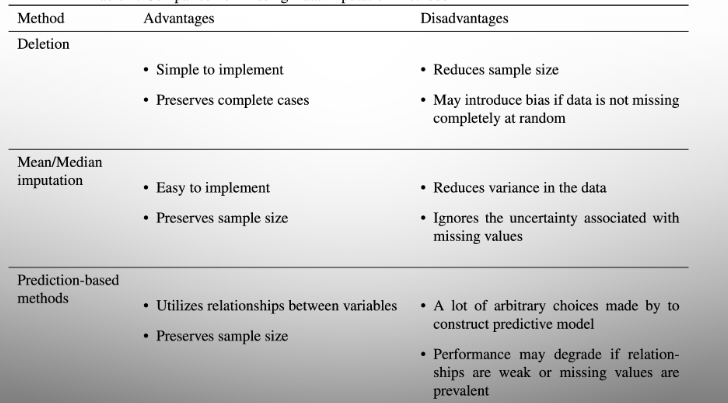
Main methods for dealing with missing data

1. Delete row with missing data

2. Insert mean value for feature data

3. Prediction based (generate a linear regression model based off other features)

Comparison of missing data methods

Outlier Data

Outliers can significantly affect the performance of our model

Outliers can arise due to:

• Measurement errors

• Data entry errors

• Malicious data poisoning

• Natural variabilities

• Rare events

To handle them

1. Treat as missing data

2. Scale appropriately

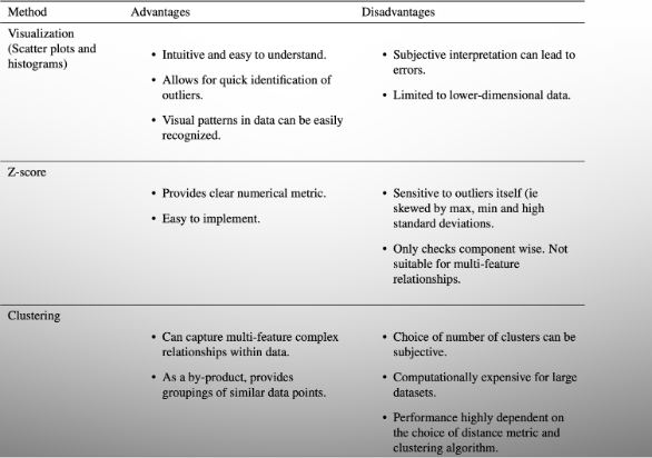
Methods for detecting outliers

1. Visualisation

   1. Scatter plots - outliers appear away from main data

   2. Histograms - outliers appear in low-frequency bins

2. Z-score

   1. Detect outliers above a threshold set after normalising the data

3. Clusters

   1. Extreme outliers may be single elements within a cluster or may be unable to find a well-fitting cluster

Comparison of Outlier Detection methods

Principle Component Analysis

A technique to reduce the dimension of the feature space by calculating the projection of the feature data onto a lower dimension.

Calculating PCA Projections

1. Compute the eigenvectors and eigenvalues of X^TX (assuming centered data)

2. Create a matrix V_q where the columns are the eigenvectors of the largest q eigenvalues

   1. The columns are the principal components

3. Compute the projection by calculating z_i = V_q^Tx_i

Bayes Classifier

Try to find a function that approximately represents

𝑓_l(𝑥) ≈ ℙ( 𝑦 = 𝑙 | 𝑥).

Now 𝑓_l(𝑥) ∈ [0,1] provides an estimate on the probability that the data sample 𝑥 is labelled 𝑦 = 𝑙

Logistic Regression

A popular choice for the probability function is the logistic function (sigmoid)

f(x) = 1/(1 + e^-x)

Likelihood Function

Aim to maximise the probability of observing the training data assuming our ML model is correct

Optimal parameters are such that l(a₀, a₁) ≈ 1 and suboptimal parameters are such that l(a₀, a₁) ≈ 0

Advantages of K-Nearest Neighbours

• Does not assume that our model, 𝑓(𝑥), takes a certain parametric structure.

• Since there are no parameters, no need to optimize.

• Can represent complex boundary conditions.

Disadvantages of K-Nearest Neighbours

• Arbitrarily chooses a metric for closeness (the Euclidean norm).

  • Depending on the units and scale of the data this may not be the best metric.

• Arbitrarily chooses 𝑘 ∈ ℕ, the size of the neighborhood.

• Only considers what is occurring locally around data point where global properties may be important.

• A lot of online computation is required to make each prediction (we are required to compute 𝑁_k(𝑥₀)).

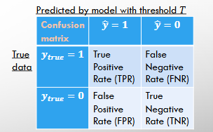
Confusion Matrix

• TPR = number of correctly predicted positive labels / number of truly positive data

• FNR = number of incorrectly predicted negative labels / number of truly positive data

• FPR = number of incorrectly predicted positive labels / number of truly negative data

• TNR = number of correctly predicted negative labels / number of truly negative data

Sensitivity and Specificity

Unlike regression models, classification problems are interested in measuring class-specific performance

• Sensitivity = TPR = percentage of positive cases correctly identified

• Specificity = TNR = percentage of negative cases correctly identified

ROC Curves

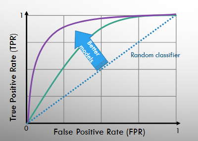
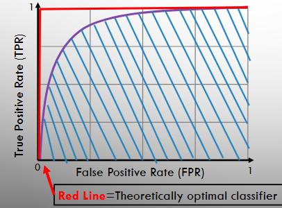
The performance of a classification model is done by plotting a Receiver Operating Characteristic (ROC) curve

• Given a classification model for different threshold values, we plot the TPR vs FPR to get the ROC curve

• We would like to find a classifier that has TPR = 1 and FPR = 0

AUC (Area Under the ROC Curve)

• Provides a metric for the performance of a classifier over all thresholds

• Theoretically the best classifier has an AUC of one

What is the main problem with collecting data

Obtaining data from a wider population is often infeasible because:

• It takes a lot of effort to collect all the data and therefore this is expensive

• It might be a rare event and therefore a lack of possible obtainable measurements

• There might be a lack of quality data

Why do we split data sets

Predicting with one data set will have no metric to assess the quality of this prediction.

If the estimates from the split data are close, we can trust our estimation.

If we only have one measurement, then we have no way of assessing how confident we should be about this estimation.

Bootstrapping

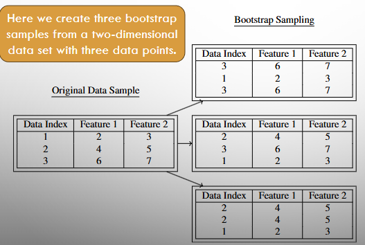
• Artificially create new data sets from a single data set by sampling with replacement.

• Sampling with replacement may cause bootstrapped samples to contain duplicate data.

  • Sometimes need to do data processing to handle this (delete / PCA)

  • If we are estimating the mean then data processing is unnecessary

• Rather than a single estimation based on the entire data set, we have a range of estimations and can say how confident we are.

How to combine Bootstrapped Models

• Known as Bootstrap, Aggregation, or Bagging

• Suppose we have a data set, and have created N bootstrapped data sets in which we have trained N models:

  • Regression - Take the average of the bootstrapped models

  • Classification - Take the majority vote of the bootstrapped models

• Bagging helps to reduce the chances of overfitting by reducing model prediction variability

  • Used for high-variability models where it is not easy to regularise

Decision Tree Terminology

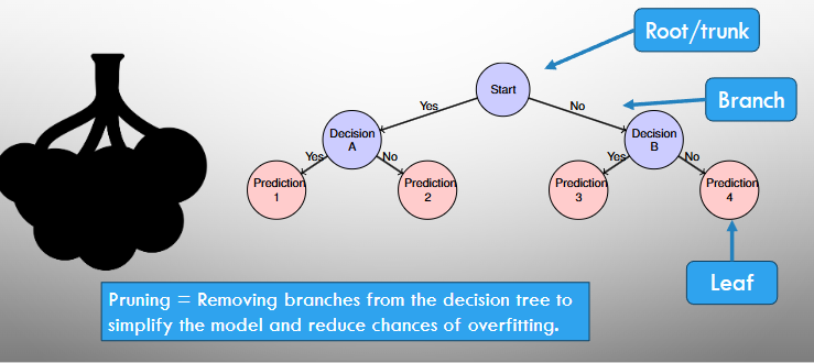
Decision Tree Visualisation

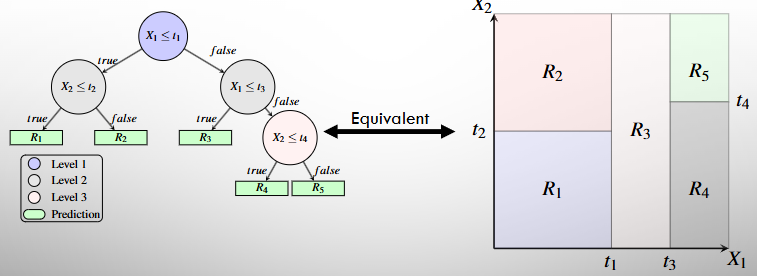
How do Decision Trees make Predictions

Suppose you have answered a sequence of binary questions for input data x and have arrived at a leaf in region R

• Regression - the average values of the labels in region R

• Classification - the most common label of feature training data in region R

Splitting the Decision Tree

• Grow trees sequentially downwards

• Grow trees greedily, so we select the leaf to split that most improves our model

• Regression - calculate the training MSE resulting for each split and choose the best

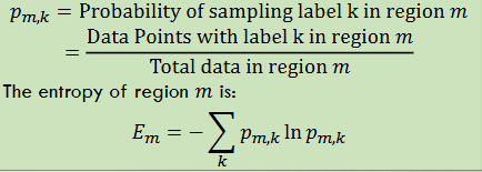
• Classification - calculate the training Entropy resulting for each split and choose the best

Entropy

The smaller the entropy, the better

Variations of Decision Trees

It is easy to overfit a decision tree (one leaf for each training data point) so we use:

1. Bag of Trees

   1. Bootstrap the training data to make multiple decision trees

   2. Average the output to make a prediction

2. Random Forest

   1. Create a bag of trees - but each tree we make our split based on only a random subset of feature variables

   2. By randomly sampling a subset of the features we give non dominant features a chance to be at the root of the tree, increasing the diversity within our bag. Therefore, our model will be less sensitive to noise within a particular feature.

SVM Definition

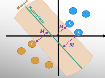
Support Vector Machine finds the hyperplane that separates binary labelled data points by maximising the margin (the minimum distance between the hyperplane and any data point)

Support vectors lie on the boundary of the margin. Therefore, changing the position of non-support vectors does not affect the optimal hyperplane.

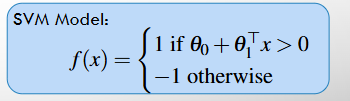
SVM Model

• Can be expanded to nonlinear decision boundaries by using basis functions

• We can solve the optimal separating hyperplane in a higher dimension and project our decision boundary back into the original dimension for nonlinear basis.

  • It is much easier to find the hyperplane that separates the points in the higher dimension

K-Means Clustering

A heuristic approach to clustering

1. Randomly assign a number from {1,…,K} to each data point

2. Iterate until cluster assignments stop changing:

   1. For each of the K clusters, compute the cluster centroid

   2. Update the cluster assignment of each data point to the cluster with the closest centroid.

May converge to a local minima rather than optimal clustering, but is more tractable to execute than brute force (K^N iterations)

Advantages of K-Means

More computationally efficient than finding the optimal clusters by brute force.

Disadvantages of K-Means

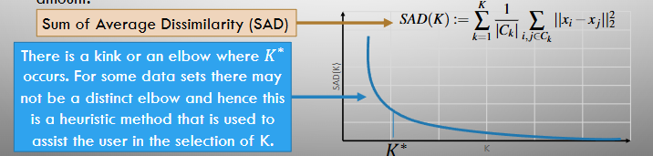
• The user must select the number of clusters, 𝐾. This is an arbitrary choice and only heuristic methods like the elbow method can be used to assist

• Does not necessarily converge to the optimal 𝐾 clusters. The local min that is outputted strongly depends on the initialization of cluster data assignment.

• Clusters all have a certain “spherical" shape, being defined by points closest to a centroid. May struggle to model clusters with more complicated shapes

Hierarchical Clustering (Dendrograms)

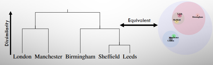
Offers a different way of grouping data without needing to decide on the number of clusters beforehand.

Gives us a highly interpretable visual called a dendrogram, which shows how data points are connected in a tree-like structure.

Hierarchical Clustering Algorithm

Greedy algorithm

1. Begin with N data points and measure the euclidean distance of all the pairwise dissimilarities

2. Iterate through i = N to 1

3. Examine all pairwise inter-cluster dissimilarities among the i clusters and identify the pair of clusters that are least dissimilar

   1. Fuse these two clusters, the dissimilarity indicates the height in the dendrogram the fusion should be placed

4. Compute the new pairwise inter-cluster dissimilarities among the remaining i-1 clusters.

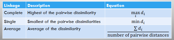
Cluster Linkage

The term used to call the dissimilarity between clusters.

To compute linkage, must compute all pairwise dissimilarities.

Elbow Method

For some data x of length N with naturally occuring clusters C₁ ,…,C_K

• When K < K^* some of the clusters will contain elements from more than one of the naturally occurring clusters and there will be high internal dissimilarity within some clusters.

• When K > K^* some of the clusters will partition one of the naturally occuring clusters and hence increasing K further will only decrease total dissimilarity by a small amount.

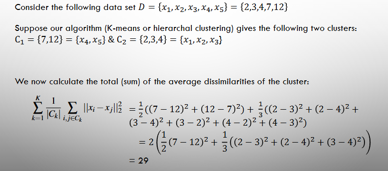
Calculating Average Dissimilarity

Ethics in ML

About value-driven decision-making, encompassing whether and how ML systems should be used, including (but not limited to) bias considerations.

Example: Deciding whether to deploy a facial recognition system at all in a public space due to concerns about privacy and mass surveillance, regardless of how biased it is.

Bias in ML

• A technical property of models that can often be measured and mitigated.

• Refers to systematic errors leading to consistent distortions in the output of a machine learning model, often resulting from inherent limitations in the data used for training or from the algorithm itself.

• Biases can lead to unfair or discriminatory outcomes, as the model may exhibit preferences or inaccuracies that disproportionately impact certain groups or individuals

• Example: A facial recognition system that performs worse on certain groups of people due to under-representation in the training data.

Types of Bias in ML

• Data Collection

  • Sampling Bias - We sample data from the wider population in a non-uniform way

  • Exclusion Bias - During data cleaning, we may wish to exclude certain features and omit some data (outliers, missing data, etc)

• Model Training

  • Technical Bias - We decide what method, type of regularization, hyperparameters, etc that all impact model output prediction.

• Model Deployment

  • Contextual Bias

    • We may misuse the model by deploying it in a way not intended during training.

    • We may selectively censor the model's output.

    • We may deploy the model in a way that does not benefit all of society equally.

• Real World

  • Real world (historical) bias - High-quality data does not exist for all groups and events equally

Techniques to Prevent Bias

To ensure your model is ethical you should create an outer feedback loop to ensure that the model is compliant with stakeholder ethical concerns.

You may make modifications to any of the stages in your ML pipeline to ensure the model is ethical.

This includes checking how the model is being used and what impact is having on certain groups.

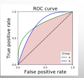
Tuning Thresholds for Fairer Models

Given a trained Bayesian binary classification model, suppose there are two groups within the training data set.

Plot the ROC curve for both groups separately.

Pick the model threshold where the model gives the same TPR and FPR for both groups.

The challenge of understanding AI decisions

• Issue: ML systems often lack explanations for their decisions

• Challenge: Understanding the logic becomes harder as we develop more powerful algorithms

• Consequence: Black box models can cause harm due to their opaque nature

Interpretability

• In safety-critical domains, such as driverless cars, ensuring human life's safety is paramount. To achieve this, it's imperative to comprehend how machine learning (ML) models arrive at their predictions. By doing so, we empower ourselves to rectify potential failure modes and make ethical decisions proactively, rather than relying solely on algorithmic outputs.

• Neural Networks (NN) exhibit remarkable capability in expressing a wide array of functions. However, deep NNs comprising thousands of neurons intricately anipulate and combine feature variables in ways beyond human comprehension

• Simpler models like decision trees provide interpretable frameworks. By tracing the path of a decision tree, we can easily deduce the logic underpinning each decision, offering valuable insights into the model's decision-making process.