CSDS 101 2nd Half
 Call Kai
 Learn
 Practice Test
 Spaced Repetition
 Match
 Flashcards
 Knowt Play
1/117

There's no tags or description
Looks like no tags are added yet.
118 Terms
machine learning
scientific study of algorithms and statistical models that computer systems use to effectively perform a specific task without using explicit instructions, relying on models and inference instead
Supervised machine learning
an expert gives the algorithm feedback on every choice the algorithm makes (ex: correct/incorrect)
unsupervised machine learning
there is no expert providing feedback. Instead the algorithm tries to “cluster” data into cohesive groups
Reinforcement algorithms
there is no expert providing feedback, but there is a general metric telling the algorithm if it is doing well or poor
classification machine learning problem
-We have two or more classes (categories). Given an instance, to which class does it belong?
-ex. Predicting whether an incoming email (instance) belongs in the "Spam" (category) folder or the "Inbox" (category) folder
regression machine learning problem
-Given an instance, what is the value for the instance?
-ex. Predicting the exact dollar value of a house based on its square footage, number of bedrooms, and zip code
ranking machine learning problem
-Given an instance, can we correctly place it into an ordered list of instances?
-Ordering millions of indexed web pages so the most helpful links appear at the top (Position #1, #2, #3) when you type a query
label
-the thing we're predicting
-ex. the future price of wheat, the kind of animal shown in a picture, the meaning of an audio clip, or just about anything
features
-input variables
-A simple machine learning project might use a single feature, while a more sophisticated machine learning project could use millions of features
-ex. If we were building an email spam detector, the features could include the following: ❖ words in the email text ❖ sender's address ❖ time of day the email was sent ❖ email contains the phrase "one weird trick.

example
a particular instance of data
labeled example
-includes both feature(s) and the label
-We can use labeled examples to train the model
-ex. full emails with “spam” or “not spam” labels
unlabeled example
-contains features but not the label
-ex. just a bunch of full emails that aren’t labelled as “spam” or “not spam”
model and its 2 phases
-defines the relationship between features and label
-ex. a spam detection model might associate certain features strongly with "spam"
-training phase: creating or learning the model. That is, you show the model labeled examples and enable the model to gradually learn the relationships between features and label.
-inference phase - applying the trained model to unlabeled examples. That is, you use the trained model to make useful predictions
each instance is a k-tuple of values
-ex. Each instance is a movie. The features are: director, the different actors, genre, year, runtime, etc. Joker = (crime, drama, superhero, actor1 = “Joaquin Phoenix”…)
-ex. 4 types of features → k=4
training/testing data
-Training data: The data we train the algorithm on. Each instance must be correctly classified by an expert. The expert value is the label of the instance.
-Testing data: Data set aside to test the algorithm on. This data must also be correctly classified by an expert.
-The training and testing data should be drawn from the same distribution.
parameters
the internal configuration variables that a machine learning model learns and adjusts from the training data to make predictions
ex. In a model predicting house prices based on square footage, the equation looks like this:
Price = (w x Square Footage) + b
The Parameters:
Weight (w): Set to $200 (meaning each square foot adds $200 to the price).
Bias (b): Set to $50,000 (the base price before adding size).
How they work: The model starts with random guesses for w and b, sees how wrong its price predictions are, and adjusts them until it finds the line that best fits the data.
Gradient descent
-over many rounds of training
-Compute the partial derivative of the error function for each parameter of f. Modify the parameter(s) with the largest partial derivatives. Repeat until error min is reached (repeat until slope goes from steep to flat)
-find the parameter and the amount to change it that makes the biggest improvement in the model’s accuracy
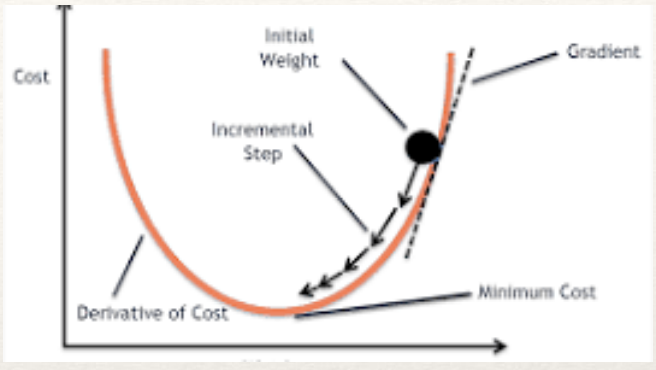
gradient descent local and global minima
local: parameter changes until it is very hard to figure out how to change the parameters to reduce the error any further
global: parameter changes that completely minimize error

generalization
-How well does minimizing the error function on the training data correspond to minimizing the error function on the test data or on real world data?
-Good generalization means it can accurately recognize a cat in a photo it has never seen
-Poor generalization usually means overfitting—where the model memorized the training set down to every minor noise or quirk, failing miserably in the real world
confusion metric
counting up the number of times a classification model gets things right and wrong (ex. classifying things as moths or not)

accuracy error metric
-Accuracy = (TP + TN) / (TP + FP + TN + FN)
-How often is the algorithm answering correctly?
precision, recall, and specificity error metrics
made possible with confusion matrix
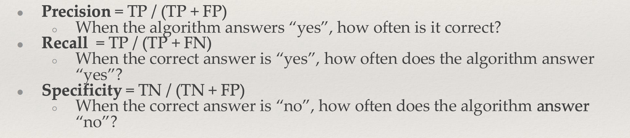
skewed distribution
-data isn’t mixed well and doesn’t reflect reality accurately
-ex. The data has ⅔ moth pictures and ⅓ butterfly pictures
It is important to look closely at the data and the confusion matrix and not just accept accuracy of the algorithm as a measure of quality
yep
overfitting
-The model does well at predicting the training set, but too well—it’s learned the peculiarities of the training set to the detriment of generalization
-Overfitting is often caused by making our model more complex than is necessary
-The fundamental tension of machine learning is between fitting our data well, but also fitting the data as simply as possible.

Ockham's Razor
The less complex an ML model, the more likely that a good empirical result is not just due to the peculiarities of the sample
Good performance on the test set is a useful indicator of good performance on the new data in general, assuming that:
-The test set is large enough.
-You don't cheat by using the same test set over and over.
Never train on test data!
-If you are seeing surprisingly good results on your evaluation metrics, it might be a sign that you are accidentally training on the test set.
-if you do this, you’re no longer accurately measuring how well the model generalizes to new data
how to prevent overfitting to the test data
-if you continuously tweak the model because it scored poorly on the test set, the test set becomes part of the development loop and the model becomes overfitted
-the validation set becomes the new test set and at the very end, you use the actual test set (you only use the test set once and use the validation set multiple times)
-pick model that does best on validation set → confirm results on test set

decision trees / attributes
-One possible representation for hypotheses
-We imagine someone taking a sequence of decisions.
-attributes are the specific questions/boolean expressions
-ex. Problem: decide whether to wait for a table at a restaurant, based on the following attributes:
1. Alternate: is there an alternative restaurant nearby?
2. Bar: is there a comfortable bar area to wait in?
3. Fri/Sat: is today Friday or Saturday?
4. Hungry: are we hungry?
5. Patrons: number of people in the restaurant (None, Some, Full)
6. Price: price range ($, ,$)
7. Raining: is it raining outside?
8. Reservation: have we made a reservation?
9. Type: kind of restaurant (French, Italian, Thai, Burger)
10. WaitEstimate: estimated waiting time (0-10, 10-30, 30-60, >60

Prefer to find more compact (simple) decision trees: we don’t want to memorize the data, we want to find structure in the data! (And remember Occam's Razor)
yep
Hypothesis spaces
-How many distinct decision trees with n Boolean attributes?
= number of Boolean functions
= number of distinct truth tables with 2^n rows
=2^2^n
-ex. with 6 Boolean attributes, there are 2^2^6 = 18,446,744,073,709,551,616 trees
choose "most significant" attribute as root of tree
-a good attribute splits the examples into subsets that are (ideally) "all positive" or "all negative"
-ex. in the picture, the patrons is a better attribute because it has the greatest Information Gain
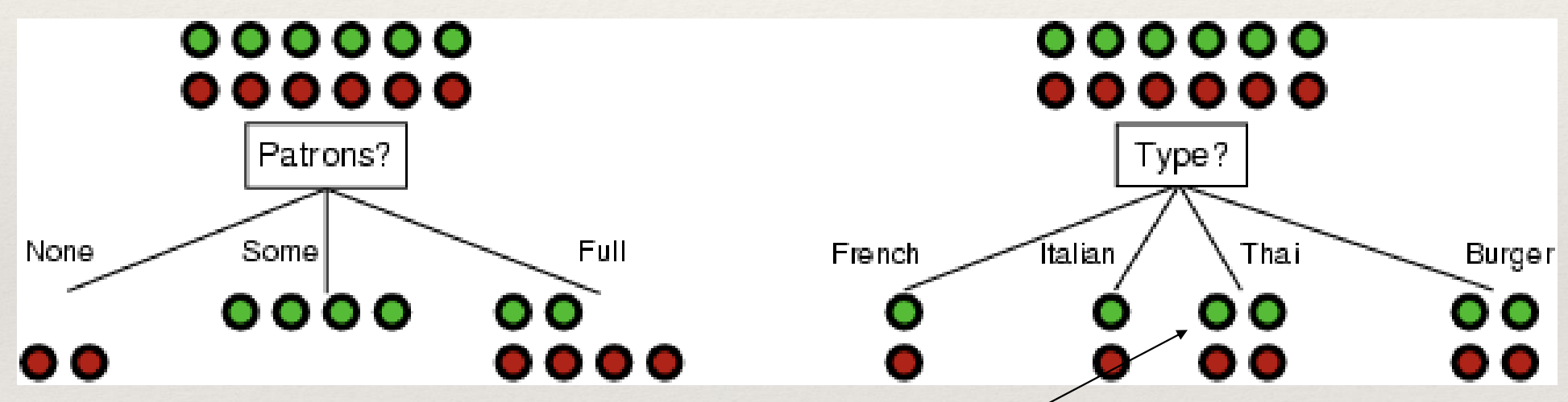
heuristics of decision tree
-If we keep going until perfect classification we might over-fit
-don’t have to use every attribute if some attributes don’t really predict much, this would just over-fit the model
-Stop when Info-Gain (Gain-Ratio) is smaller than threshold
-Stop when there are M examples in each leaf node (ex. people who passed exam after being tutored is 4 and people who failed is only 1, so we can say that this attribute doesn’t really matter that much because number of examples was only 1 for failing exam)
pruning
Sometimes it is better to grow the trees all the way down (use all attributes) and prune them back later (remove some insignificant attributes). Later splits may become beneficial, but we wouldn’t see them if we stopped early
random forest
-grow many trees on random, sub-datasets sampled from the original dataset
-each tree contains different attributes (ex. to decide if a movie will be liked by someone, one tree can have attributes of movie director and genre and another tree can have attributes of movie length and actors)
-based on what a majority of the trees conclude, decide the overall answer (ex. if 70% of trees said the person would like the movie, the final output is that they will like it)
Linear ML

empirical risk minimization
-Training: learning (determining) good values for weighs and bias from labels examples -Supervised Learning: builds a model by examining lots of labeled examples to find a model that minimizes loss (the penalty for bad predictions)
loss
-The arrows represent loss.
-The blue lines represent predictions.
-High loss on the left model; low loss on the right model.

Calculating Loss
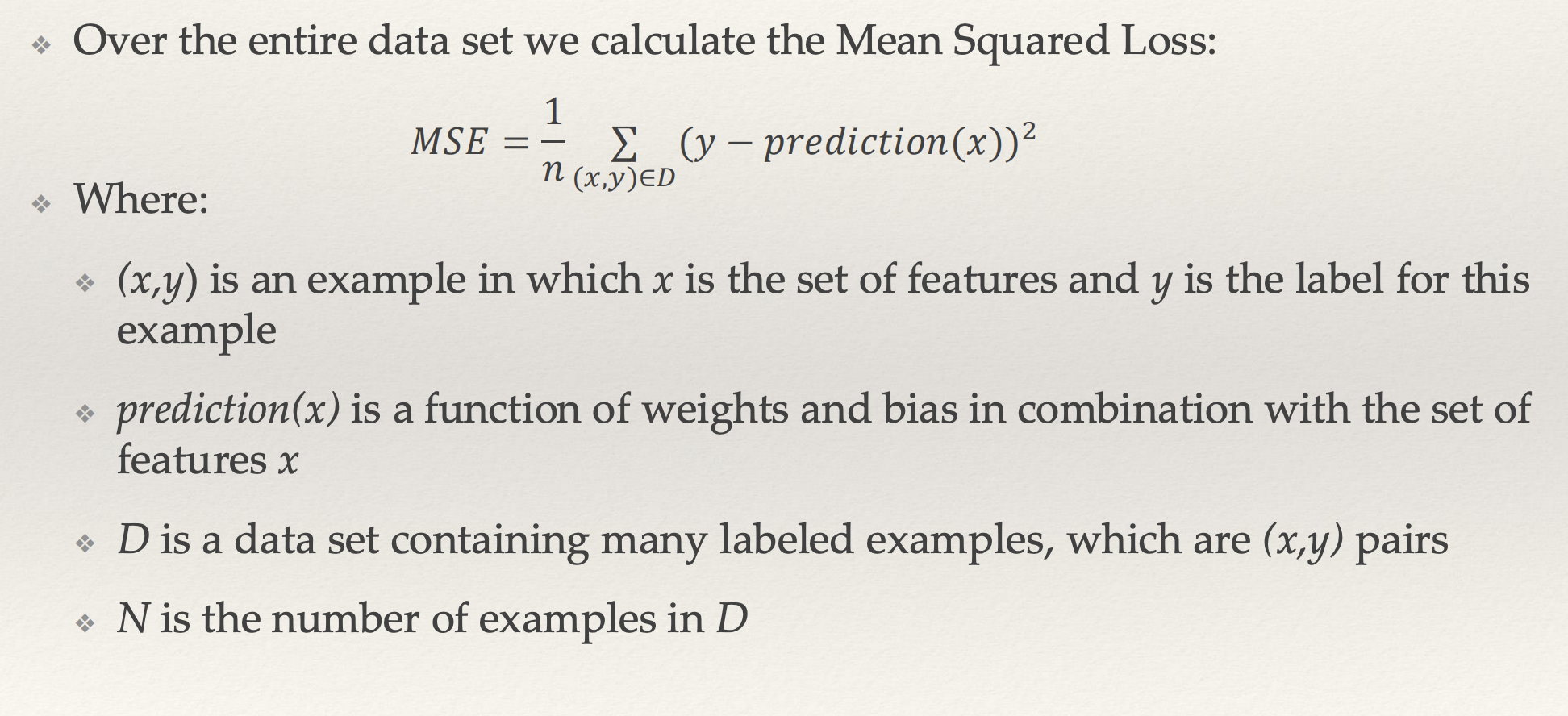
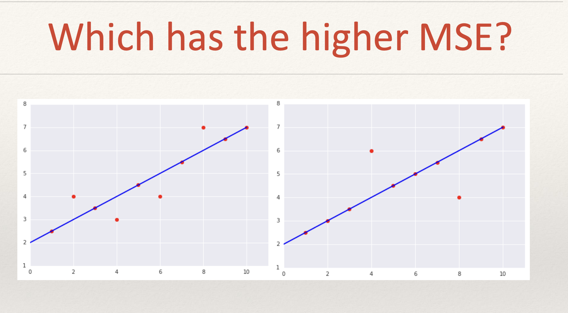
graph 2
graph 1: 1/10 (1+1+1+1) = 0.4
graph 2: 1/10 (2² + 2²) = 0.8
learning rate
-size of the adjustments to weights/bias to reduce loss and move from steep to flattest part of gradient descent graph
-bigger adjusts = higher learning rate
-don’t want adjustments to be too small or too big

Support Vector Machines
-Typically used for classification
-Given a set of n points in a k-dimensional space, find a hyperplane that separates the two classes.
-What if no such hyperplane? Map the instances to a higher dimensional space (the mapping does not have to be linear) and find the hyperplane in that higher dimensional space
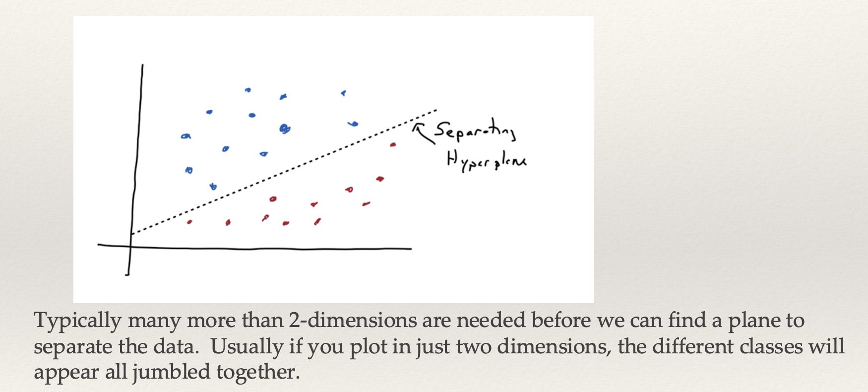
linearly separable
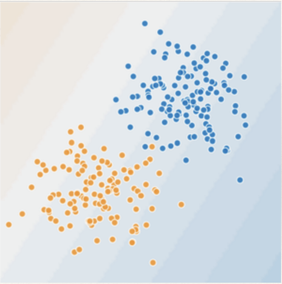
not linearly separable

feature cross
-Address non-linearity by adding a new feature to the data set
-Say we originally have 2 features: 𝑥1 and 𝑥2
-We could add a third synthetic feature that encodes the nonlinearity as a product of those features: 𝑥3 = 𝑥1𝑥2 that encapsulates how feature 1 and 2 interact to affect trends
-Then our linear learner can go about its business learning the weights for: 𝑦 = 𝑏 + 𝑤1𝑥1 + 𝑤2𝑥2 + 𝑤3𝑥3
ex. If an online retail app wants to predict whether a user will buy a premium item, treating the user's demographic group and the time they are shopping independently misses the magic window when shopping actually happens.


Activation Functions
-Each neuron multiplies incoming inputs by weights, adds a bias (z = wx + b), and passes the result forward. An activation function (a = f(z)) bends or folds the straight-line math.
ReLU (Rectified Linear Unit): Outputs the input directly if it is positive (x > 0), and zero otherwise

nonlinear model example:
Step 1: The Input Layer (Raw Features)
The data for our house is normalized and loaded directly into the three input nodes:
x1 (Size): 0.9
x2 (Bedrooms): 0.4
x3 (School Rating): 0.8
Step 2: Hidden Layer 1 (Feature Extraction)
Both hidden nodes look at all three inputs, but because they have different weights, they calculate completely different things.
🔹 Hidden Node 1 (Focuses heavily on Size & Bedrooms)
Weights: w = [1.0, 0.5, -0.1] | Bias: b = -0.2
Weighted Sum (z1): (0.9 x 1.0) + (0.4 x 0.5) + (0.8 x -0.1) + (-0.2) = 0.9 + 0.2 - 0.08 - 0.2 = 0.82
Activation Output (a1): ReLU(0.82) = 0.82
🔸 Hidden Node 2 (Focuses heavily on School Rating)
Weights: w = [-0.2, 0.1, 1.2] | Bias: b = -0.5
Weighted Sum (z2): (0.9 x -0.2) + (0.4 x 0.1) + (0.8 x 1.2) + (-0.5) = -0.18 + 0.04 + 0.96 - 0.5 = 0.32
Activation Output (a2): ReLU(0.32) = 0.32
The outputs from this layer (0.82 and 0.32) now become the new inputs for the next layer.
Step 3: The Output Layer (Final Decision)
Our single output node takes the signals from the two hidden nodes, applies its final weights, and uses Sigmoid to compress the result into a final prediction percentage.
Incoming Signals: a1 = 0.82, a2 = 0.32
Output Node Weights: w = [0.8, 0.4] | Bias: b = -0.3
Weighted Sum (z out): (0.82 x 0.8) + (0.32 x 0.4) + (-0.3) = 0.656 + 0.128 - 0.3 = 0.484
Activation Output (a out): Sigmoid(0.484) = 0.619
🎯 The Verdict
The model outputs 0.619. This means it calculates a 61.9% probability that this specific house falls into the "High Price" category.

neural net
-A set of nodes, analogous to neurons, organized in layers (A biological neuron receives chemical or electrical signals through its branch-like dendrites. An artificial node receives numerical data inputs from previous layers in the network)
-each hidden node has a set of weights, a bias, and an activation function
-each input node contains a single feature
-Very versatile algorithm that can be used for classification, regression, or distribution discovery (but here we are focusing on classification)

how many input, hidden, and output nodes must a neural network have?
Input layer: one “node” for each feature of the input, or for pictures, one “node” for each pixel of the input.
Hidden layer: the number of nodes is up to the neural network designer
Output layer: For classification into two classes, only one output node is needed. Its value is 1 for the “yes” class and 0 for the “no class (ex. cat or not). For classification into many classes, one output node per class. A node’s value is 1 if the input belongs to that class and 0 if not (ex. cat or dog, one node for cat or not and another node for dog or not).
A large positive or negative weight means that this input variable counts a ___ (positively or negatively) to the output, a small weight means the input counts a ___ to the output
lot, little
Training the neural network is to find the best weights a node should use for each input to that node in order to achieve the desired output
yep
Back propagation
The gradient descent algorithm for neural networks.
It looks at the output values to see how correct (or wrong) they are.
Then distribute the correctness/error value to the hidden layer nodes based on the weights of the values to each output. (How much did each input to the node contribute to that node’s value)
Using derivatives on node’s function, determine how much to adjust the weights that the node uses in its function
How Decision Trees and Neural Networks are Similar?
-both can be used for classification and regression
-both transform inputs and map them to outputs
-both are layered
Where is the Information Stored in a Neural Network?
distributed globally in the weights and biases
specialized hidden layer types: convolution and pooling
-“Convolution layers”: collect inputs that correspond to regions on an image and apply specialized “masks” (fixed weights on the inputs)
-“Pooling layers”: reduce the number of nodes in a hidden layer by collecting several nodes of the previous layer and taking their maximum value or average value.
ResNet 50
A 50 layer deep learning neural network
-50,176 input nodes (for a 224x224 pixel image)
-1000 output nodes (to classify 1000 different types of images)
-A combination of different types of hidden layers (Fully connected “normal” hidden layers, Convolution layers with different “masks”, Pooling layers)
ML bias Problem
Machine learning will find patterns in data including patterns that we do not want (ML are trained on human data, so it is bound to be biased) (ex. criminal justice system biased against black men)
deep learners
-neural networks with many hidden layers
-Deep learners are very, very good at finding patterns, but the pattern the deep learner finds may not be the pattern we want it to find!
What type of ML algorithm is decision tree learning?
supervised learning
What is a random forest?
A set of decision trees that each learn a model of the data and vote on the final classification
what does ANN stand for?
Artificial Neural Network
How do ANN's model non-linearity?
By using different types of activation functions
What's the name of the ANN algorithm for updating weights in the system?
back propagation
What is deep learning?
Using a network that has a large number of hidden layers
What is deep learning primarily based on?
neural networks
Which of the following is a common activation function used in deep learning?
sigmoid, ReLU
clustering systems
-Unsupervised learning
-Detect patterns in unlabeled data (E.g. group emails or search results, find categories of customers, detect anomalous program executions, etc.)
-Useful when don’t know what you’re looking for
-Requires data, but no labels
-Often get gibberish
data sets
matrices containing lots of data points

2 main Types of Clustering Algorithms: hierarchical and non-hierarchical
Hierarchical algorithms: a. Start with each point in its own “cluster”. b. Merge clusters that are close to each other c. Repeat until we have a “good” set of clusters.
Non-hierarchical algorithms: a. Decide how many clusters we want. b. Start with a set of cluster choices. c. Put each point in the cluster it is closest to d. Adjust the clusters. e. Reassign the points based on the new clusters f. Repeat
Main Questions When Clustering
1. How to represent clusters of multiple points (clusters) ?
2. How do we decide if clusters (points) are close to each other?
3. How do we decide when to stop because the clusters are good enough?
No right answer
What could “similar” mean in clustering?
One option: small (squared) Euclidean distance

k-means clustering
an unsupervised machine learning algorithm that divides unlabeled data into k distinct groups by minimizing the distance between data points and their cluster centers
Initialization: Choose k (the number of clusters) and randomly place k initial points called centroids in the data space. [1, 2]
Assignment Step: Calculate the Euclidean distance from each data point to every centroid, and assign each point to its closest centroid. [1, 2]
Update Step: Recalculate each centroid's position by taking the average (mean) of all data points assigned to that cluster. [1, 2]
Repeat: Keep alternating between the assignment and update steps until the centroids stop moving or a maximum number of iterations is reached
trying to reduce total distance (phi)

why k-means is non-deterministic?
primarily because of its random initialization step
Random Centroids: At the start of the algorithm, initial cluster centers (centroids) are chosen randomly from the data space or selected as random data points.
Local Minima/optimum: Because K-means uses an iterative gradient-descent-like process to minimize within-cluster variance, different starting points can cause the algorithm to converge on different local minima/optimum rather than the true global minimum/optimum
Varying Results: Running the algorithm twice on the exact same dataset with different random seeds or default settings can yield different cluster assignments and centroid positions.

K-Means Questions
Will K-means converge?
To a global optimum?
Will it always find the true patterns in the data?
If the patterns are very clear?
Will it find something interesting?
Do people ever use it?
How many clusters to pick?
tokens
Computers do not process English words directly. Text is segmented into subword chunks called tokens (typically 3–4 characters or common syllables)
1,000 tokens ≈ 750 English words

vectors
Each integer token ID is converted into a vector of numbers in a high-dimensional continuous space. Semantically related tokens occupy nearby coordinates

Vocabulary Size (V)
Modern LLMs operate over fixed vocabularies of approximately 50,000 to 100,000 unique token pieces
LLMs don’t ”think” they predict the next likely unit of text based on massive patterns and probabilities
yep
logit
-used when trying to figure out next word in sentence
-The final layer of the neural network scans its entire vocabulary (tens of thousands of words) and assigns a raw score—a logit (𝑧𝑖 )—to every possible next word
-scores aren’t yet useable probabilities
-ex. "The cat sat on the..."
Candidate Word | Raw Logit Score |
|---|---|
mat |
|
floor |
|
couch |
|
dog |
|
banana |
|
softmax
-used to convert logits to actual percentages
-the model passes these raw logits through the Softmax function, which converts them into clean percentages that sum to 100%
-ex. "The cat sat on the..."
Candidate Word | Raw Logit Score | Final Probability |
|---|---|---|
mat |
| 72.3% |
floor |
| 19.7% |
couch |
| 6.6% |
dog |
| 0.2% |
banana |
| ~0.0% |

temperature
-Way to alter probabilities of next words a bit by changing the “temperature” of the system (T>0)
-T alters probability curve
-Low Temperature (T ≈ 0.1 – 0.3) - Greedy / Focused, Sharply favors top-ranked tokens. High reproducibility; ideal for code and structured math.
-Moderate Temperature (T ≈ 0.7) - Standard Chat, Balances coherence and stylistic diversity. The typical default for conversational AI.
-High Temperature (T > 1.0) - Creative / Unstable, Flattens the probability curve. Increases novelty but dramatically increases hallucination risk.
-higher the temp., the more the probabilities all become closer to each other
-weights of the model and calculated raw logits don’t change with temp.
-Temperature is simply an inference-time decoding knob that dictates how boldly or cautiously the system rolls the dice when picking the next token from that distribution
-ex.
Candidate Word | Raw Logit | Scaled Logit (T = 2.0) | Default Prob. (T = 1.0) | High-Temp Prob. (T = 2.0) |
|---|---|---|---|---|
mat |
|
| 72.3% | 46.4% |
floor |
|
| 19.7% | 24.2% |
couch |
|
| 6.6% | 14.0% |
dog |
|
| 0.2% | 2.3% |
banana |
|
| ~0.0% | 0.1% |

Feed-Forward ANN
-It looks at every single word completely alone. When it sees the word "bank", it cannot look left or right to see if the sentence is about money or a river
-Once training finishes, the weights are frozen. The network cannot dynamically adjust how it processes a word based on what other words appear around it in a new sentence
Convolutional Networks (CNNs)
-It can only see 3 or 4 words at a time as it slides across the page. It catches short phrases like "coffee maker", but it loses track of words further back in the sentence
-fail when related words are far apart
Transformer model / Self-Attention Solution
-calculates dynamic affinity weights (how much one word should pay attention to another) between every word and every other word in parallel
-Dynamic Routing: Instead of static weights, connection strengths change based on the sentence itself (ex. In "The animal didn't cross the street because it was too tired", the word "it" dynamically routes strong attention to "animal". If "tired" changes to "wide", "it" shifts its attention weight to "street")
-Full Parallelism: Unlike sequential recurrence, all tokens are processed simultaneously on GPUs
-Takeaway: Attention transforms static token IDs into rich, context-aware vector representations. Attention is a dynamic weight matrix computed on the fly, not a hardcoded decision tree rule
The Three-Stage Pipeline: From Raw Web to Assistant:
Self-Supervised Pre-Training (unsupervised learning)
-Trained on trillions of unlabeled web tokens. The model hides the next token and updates weights using Cross-Entropy Loss (measures how much probability the model assigned to the true next token, penalizing low confidence and pushing the weights to increase the true token's logit next time) via massive parallel gradient descent
-ex. Given "The capital of France is", the model tries to predict the next token, uncovers "Paris", and grades itself automatically
-High world “knowledge,” but poor conversational compliance (ex. If you ask a raw base model "What is the capital of France?", it might respond with "What is the capital of Germany? What is the capital of Spain?" because its training data contains many geography quizzes formatted as lists of questions rather than helpful assistant answer)
-This stage accounts for around 99% of total computational resources
The Three-Stage Pipeline: From Raw Web to Assistant:
Instruction Fine-Tuning (SFT) (supervised learning)
-Curated dataset of prompt-and-response pairs crafted by human experts. Teaches the model the structure of questions, answers, and coding tasks
-Understands conversational role-playing and direct user prompts
-why this improves stage 1:
Pure Pattern Extension: If you feed a base model a prompt written in a specific voice, it predicts the next tokens as if the same author is still typing.
No Conversational Boundary: Because it lacks special chat tokens (like
<|user|>and<|assistant|>), it does not recognize that it is supposed to stop, switch roles, and answer you.
-ex. Suppose a user inputs the prompt: "Write a Python function to reverse a string."
Base Model (Pre-Trained Only):
Might output "Write a Python function to sort a list. Write a Python function to find a prime number." It treats your prompt as the start of a homework worksheet and keeps generating more questions.
SFT Model (Instruction-Tuned): Recognizes the
<|user|>instruction boundary, switches into the<|assistant|>persona, and outputs clean, runnable Python code followed by an explanation.
The Three-Stage Pipeline: From Raw Web to Assistant:
Reinforcement Learning from Human Feedback (RLHF)
-Human evaluators rank model outputs; a reward model steers behavior toward helpfulness and safety.
-Aligns probability distribution away from toxic or evasive answers.
The Ethics of LLMs
-Software feels weightless, but massive models operate on tens of thousands of dedicated GPUs clustered in gigawatt data centers
-Water Consumption: Millions of liters of cooling water evaporated during training and high-volume query serving.
-Energy Demands: Sustained megawatt energy draws impacting regional utility grids.
-Intellectual Property: Scraping creative works without creator attribution or compensation.
What mathematical function does an LLM use to turn its raw, unconstrained output scores (logits) into a valid probability distribution?
softmax
When you turn down the temperature slider (e.g., from T=1.0 to T=0.2) when querying an LLM, what is actually happening under the hood?
The underlying weights stay unchanged; the model simply becomes more focused/greedy when picking tokens.
If you are using an LLM to write syntactically strict Python code or solve structured math equations, which temperature setting is most appropriate?
Low temperature (T~0.1-0.3)
Why did Transformer models replace older Convolutional Networks (CNNs) for largescale language processing?
CNNs rely on small local filters and fail to connect related words that are far apart.
Which stage of the modern LLM pipeline accounts for roughly 99% of the total compute resources?
Self-Supervised Pre-Training on trillions of web tokens
What is the primary purpose of Reinforcement Learning from Human Feedback (RLHF) in the 3-stage LLM pipeline?
Steering model behavior toward helpfulness, safety, and non-toxic outputs using human preference rankings.
Even though digital software can feel 'weightless', why do modern LLM data centers have substantial real-world physical footprints?
They require millions of liters of cooling water and sustained megawatt power grids to run GPU clusters.
survivorship bias
Data is biased toward those entities that are still here. The ones that fail should also concern us
ex. The military was only plotting bullet holes on the planes the survived. They had no data on the planes that did not make it back. Don’t add armor where the bullet holes are. Add it where they are not.
ex. People often study billionaire entrepreneurs or college dropouts (like Steve Jobs or Bill Gates) and assume that quitting school or taking massive risks is the secret to wealth. This ignores the thousands of people who tried the exact same thing and went bankrupt.
Conditional Probability
-Pr (Outcome | Event) = what is the probability that the outcome occurs given that the particular event occurs.
-used to determine if an algorithm is fair
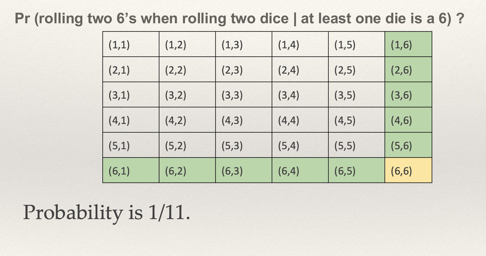
group fairness
-The probability of an outcome is the same across all groups.
-Formally, for any two groups A and B: Pr (Outcome = 1 | Group = A) = Pr (Outcome = 1 | Group = B)
-If the conditional probabilities are different, then the data may be biased toward a particular group.
-Ex: Compas system did not satisfy group fairness when the groups are races