Micro Unit 2

Law of Demand

• inverse relationship between price and quantity demanded

Ceteris paribus

• “all other things held constant” —> when reading a demand curve, assume all outside factors are held constant

Change in price

• movement along the curve; no shift

• the only thing that c an change the “quantity demanded”

Change in demand

• shift right or left

Demand Shifters

1. Tastes and Preferences

2. Related Goods (price of)

3. Income

4. Buyers (number of)

5. Expectations

Tastes and Preferences

• more popular —> shifts right

• less popular —> shifts left

Substitutes

• price increases —> demand increases, shift right

• price decreases —> demand decreases, shift left

Complements

• price increases —> demand decreases, shift left

• price decreases —> demand increases, shift right

Buyers

• increase in number of consumers —> shift right

• decrease in number of consumers —> shift left

Normal goods

• income increases —> demand increases

• income increases —> demand increases

Inferior goods

• income increases —> demand decreases

• income decreases —> demand increases

Expectations

• if consumers expect the price to rise later, they are more likely to buy now —> demand increases, shifts right

• expect the price to decrease later, more likely to wait —> demand decreases, shifts left

The Law of Supply

• direct relationship between price and quantity supplied

Supply Shifters

1. Inputs (price and availability)

2. Related goods (price of)

3. Expectations of Future Profit

4. Numbers of Producers (more producers = supply increases)

5. Technology (better technology = supply increases)

Substitutes for Supply

• if the price of a substitute increases, the supply with decrease for the other good

Expectations

• price of a good is expected to increase —> supply with decrease in anticipation of future prices

Elastic Demand

• consumers are highly responsive to changes in price

• price increases —> quantity demanded decreases

• price decreases —> quantity demanded increases

• greater than 1

Inelastic demand

• consumers do not respond very much to changes in price

• price increases —> quantity demanded falls a little

• price deceases —> quantity demanded decreases a little

• less than 1

Total Revenue - Inelastic Demand

• price increase —> TR increase

• price decrease —> TR decrease

Total Revenue - Elastic Demand

• price increase —> TR decrease

• price decrease —> TR increase

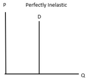
Perfectly Inelastic

• PED = 0

Perfectly Elastic

• PED = infinity

Percent Change

(New - Old)/Old * 100

Price Elasticity of Demand/Supply

% change Q / % change P

Characteristics of Goods/Services with Elastic Demand

1. Substitutes

2. Proportion of Income

3. Luxury or Necessity

4. Addictive or Habit Forming

5. Time (not in a hurry to purchase)

Characteristics of Goods/Services with Inelastic Demand

1. Few Substitutes

2. Necessities

3. Small portion of income

4. Required now, rather than later

Unit Elastic

• PED = 1

Cross-Price Elasticity of Demand (XED)

• shows if two goods are substitutes or complements

• positive —> substitute

• negative —> complements

• XED = % change in Q of good A / % change in P of good B

Income Elasticity of Demand (YED)

• shows if a good is normal or inferior

• positive —> normal

• negative —> inferior

• YED = % change in Q / % change in Y

Income-elastic

• income rises —> demand for income-elastic goods rises faster than income (+>1)

Income-inelastic

• income rises —> demand for income-inelastic goods raises, but slower than income (+<1)

Regressive

high-income taxpayers pay a smaller percentage of their income than low-income taxpayers

Proportional/flat

all taxpayers pay the same percentage of their income

Progressive

high-income earners pay a large percentage of their income

Excise Tax

a “per-unit” tax placed on the sale of a specific good of service

• shifts the supply curve to the left

• both buyers and sellers share the burden of an excise tax

• tax revenue —> box formed from the line of a tax wedge

  • amount of tax paid by consumers top half, amount of tax paid by producers bottom half

Total Expenditures

Total amount of money buyers spend on a good

• Pe * Qe

Total Revenue for firms after excise tax

New Producer Price * New Quantity

Total Expenditures after excise tax

New Consumer Price * New Quantity

Tax Incindence

Who bears the burden of a tax?

• more inelastic —> pays more burden

• demand and supply have the same elasticity —> buyers and sellers share the tax equally

Find Tax Incidence from a graph

• difference between new price after tax and price at equilibrium

Subsidy

Government payment to producers/consumers

• lowers cost of production/consumption + encourages greater production/consumption of a good/service

• shifts supply curve to the right

Price Ceiling

Government-imposed maximum price

• binding —> must be placed below equilibrium price

• help consumers by keeping prices low —> shortage because Qd>Qs

Price Floor

Government-imposed minimum price

• binding —> must be placed above equilibrium price

• help producers by keeping prices high —> surplus because Qs>Qd

Price Controls

• price floor + price ceiling

  • both result in a misallocation of resources

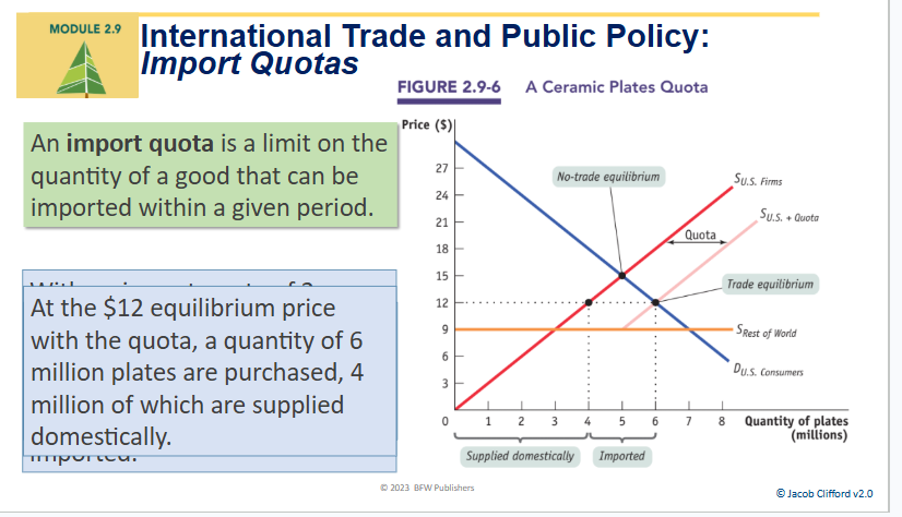
Quantity control/quota

• upper limit on the quantity of some good that can be bought/sold

• buyers pay more than what sellers would normally accept at a quote of 8 million rides

Quota rent

• difference between demand and supply price at the quota amount

International Trade/tariffs

• consumers benefit from international trade

• tariffs create deadweight loss by causing a decrease in total surplus

Domestic Price

• price of a good within a country

World Price

• price of a good on the international market

• lower than domestic price —> incentive to import

• higher than domestic price —> incentive to export

Protectionism

• government restricts international trade to protect domestic industries from foreign competition

Import Quota

• tax on imports