Chapter 5: Individual and Market Demand

Substitution vs income effect

1. Sub: the change in the QD bc a price change changes the attractiveness of substitute good

2. Income: the change in QD bc a price change causes a change in purchasing power

Market demand curve

Shows how much of a good the market as a whole wants to purchase at various prices

Price consumption curve (PCC)

• Holding income + the price of Y constant (+ preferences)

• the PCC for a good X is the set of optimal bundles traced on an indifference map as the price of X varies.

• In simple terms: a curve joining optimal consumption bundles as the price of one good changes.

What is held constant when deriving a PCC?

1. Income

2. Price of the other good

3. Preferences

Purpose of a price consumption curve (PCC)

• Shows how a consumer's optimal bundle changes when the price of 1 good changes

• Holding income, preferences and other prices constant.

• Key distinction: The PCC plots optimal bundles of TWO quantities (x + the composite good) as price changes

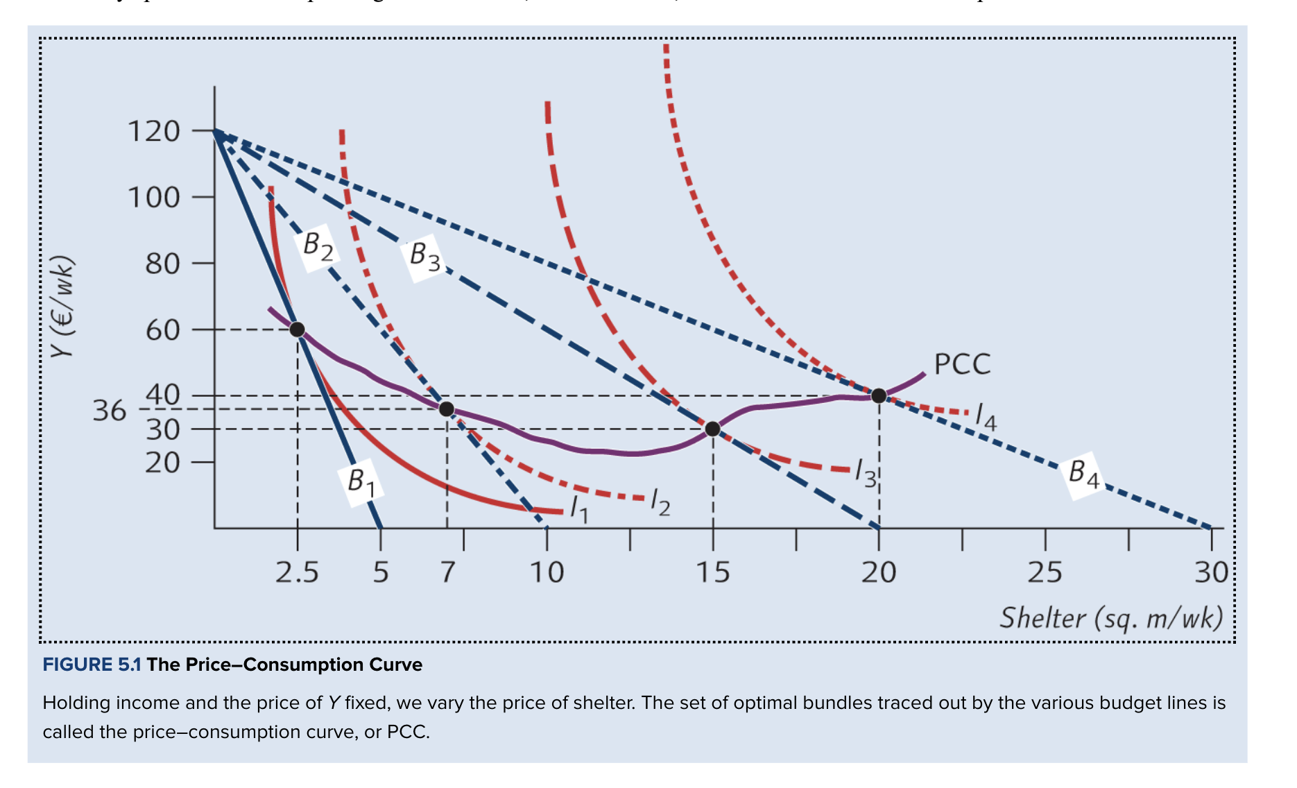
How to draw a PCC

1. Draw the indifference map and initial budget constraint

2. Good X on x axis, composite good Y on y axis

3. Change the price of good X (keep income + the price of the composite good constant)

4. The budget constraint rotates bc the price of X changes.

5. Find the new optimal bundle at each price (where the BL is tangent to an IC).

6. Join the optimal bundles to form the PCC

Draw the PCC for this.

Income: $120/week

Price of composite good: $1/unit

- When the price of shelter falls:

• The budget constraint rotates outwards around the vertical intercept.

• The consumer can afford more shelter.

• In this example, the consumer chooses more shelter at every lower price.

• Consumption of the composite good can increase or decrease.

*revisit this example

In a PCC, when varying the price of a good why is the vertical intercept unchanced?

Bc income + price of composite good remain constant

Individual demand curve

Shows quantity of a good 1 consumer will buy at diff prices, holding other factors constant

How to construct an individual demand curve? (PCC → IDC)

Can get all info from the PCC:

1. Take each optimal bundle on the PCC

2. Record the P + QD at that price

3. Plot: price on y axis & quantity on the x axis.

4. Join points

Derive the indivudal demand curve from this PCC

What is the key difference between the PCC and demand curve?

• PCC: shows quantities of 2 goods

• DC: shows price vs quantity of 1 good

• Both: summarise consumers purchase decison in response to changes in PRICE

Feature	PCC	Individual demand curve
Vertical axis	Quantity of composite good (Y)	Price of X
Horizontal axis	Quantity of X	Quantity of X
Shows	Optimal bundles as price changes	QD at different prices

Tools that summarise consumers purchase decisions in response to changes in price vs income

Price	Income
Price consumption curve (PCC)	Income consumption curve (ICC)
Individual demand curve	Engel curve

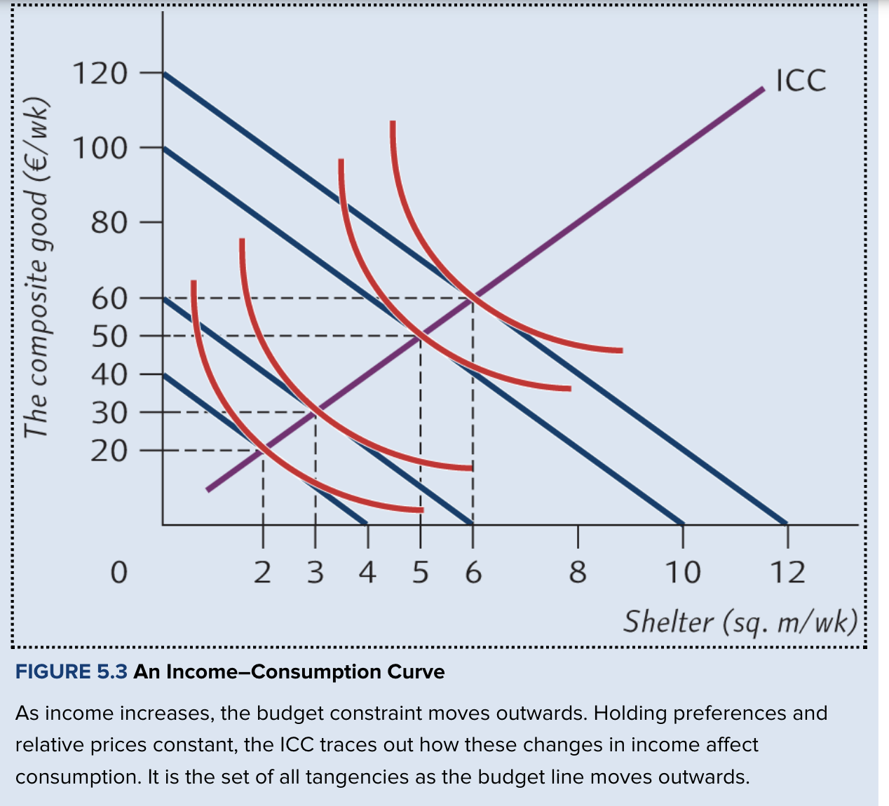
Income consumption curve (ICC)

• The ICC for a good X is the set of optimal bundles traced on an indifference map as income varies

• Holding the prices of X and Y constant

• In simple terms: shows how a consumer's optimal consumption bundles change as income changes

What is held constant when deriving the ICC?

• Preferences

• Relative prices

PCC vs ICC

How consumers optimal bundle changes with…

• PCC: price changes

• ICC: income changes

Aka how changes in price vs income affect consumption

What happens to the budget constraint when income rises?

• Shifts parallel outwards

How to construct an income consumption curve (ICC)?

1. Draw the budget constraint and indifference map.

2. Increase income, shifting the budget constraint parallel outwards.

3. Find the optimal bundle at each income level.

4. Join the optimal bundles (at the diff income levels) to form the ICC

Shape of ICC

Straight or curved

Draw an ICC using this info:

• Price of composite good: $1/unit

• Price of X: $10

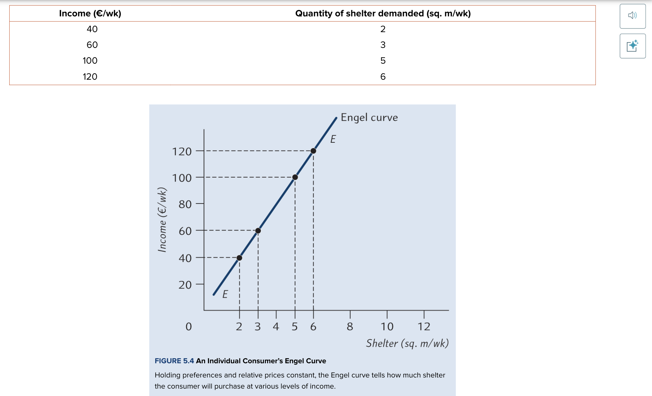
• Vary income: 40, 60, 100, $120/week

Engel curve

A curve that plots the relationship between the quantity (of good x) consumed and income

• Quantity on x axis

• Income on y axis

• Shows how QD changes as income changes

• Hold preferences and relative prices constant.

How to construct an engel curve?

Take all info from the ICC:

1. Record the quantity of good x consumed at each income level (at the optimal level)

2. Plot income on y axis & QD on x axis.

3. Join the points to form the Engel curve

for this example: As income rises, shelter consumption rises.

What does an individual engel curve show us?

How much of good x a consumer wil buy at diff income levels

Axes of ICC vs engel curve

Curve	Vertical axis	Horizontal axis
ICC	Spending on all other goods (composite good) (per week)	Quantity of good X
Engel curve	Total income (per week)	Quantity of good X

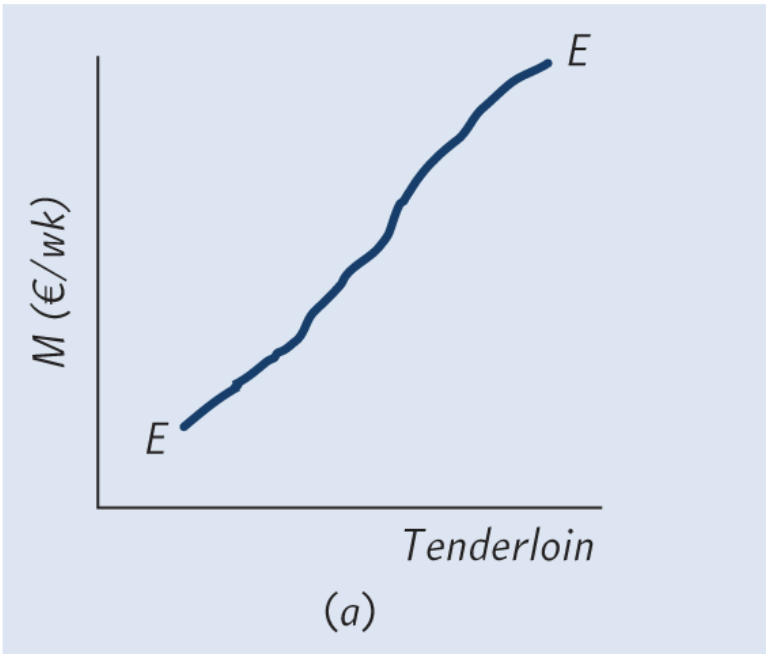
Does an engel curve slope upwards or downwards?

Either

• Depends if it is a normal or inferior good

Normal good

Good whose quantity demanded increases as income increases

• Engel curve slopes upwards

Inferior good

Good whose quantity demanded decreases as income increases

• Engel curve slopes downwards

Why might a good be inferior?

When income rises, consumers may switch to more desirable, more expensive substitutes

Can all goods be inferior for a consumer who spends all their income?

No

• They can’t spend less on every good when income rises

• The broader the category, the less likely a good is to be inferior (eg meat)

What is the key difference between the ICC and Engel curve?

• ICC shows optimal bundles of two goods

• Engel curve shows income versus quantity demanded.

2 reasons why a change in price affects quantity demanded?

1. Substitution effect

2. Income effect

Substitution effect

Change in QD bc a change in price changes the relative attractiveness of other goods (substitute goods)

What happens to QD if prices increase (substitution effect)

1. Increase price →

2. Close subs become more attractive than before

3. QD decreases

Which way does the substitution effect move quantity demanded?

QD moves in opp direction to price change

• Eg P increase → QD decrease

Income effect

Change in QD bc a price change causes a change in real purchasing power (real income)

What happens to purchasing power when prices increase and decrease?

• Price ↑ → purchasing power ↓.

• Price ↓ → purchasing power ↑.

What does the direction of income effect depend on?

If the good is normal or inferior

What happens to QD if prices increase (income effect)

1. Prices increase

2. Real income / purchasing power falls

3. If normal good: QD decreases

4. If inferior good: QD increases

How do price decrease effect normal vs inferior goods (only income effect)

1. Normal: increase PP → increase QD

2. Inferior: increase PP → decrease QD

Total effect

Substitution effect + income effect

Total effect table

Good	Substitution effect	Income effect	Relationship
Normal	Price rises → quantity falls	Quantity falls	Reinforce each other
Inferior	Price rises → quantity falls	Quantity rises	Oppose each other

How does a price rise affect demand for a normal good?

1. Substitution effect: ↑P → ↓QD

2. Income effect: ↑P → ↓QD

3. Both effects decrease QD → total effect: QD ↓

How does a price rise affect demand for a inferior good?

1. Substitution effect: ↑P → ↓QD

2. Income effect: ↑P → ↑QD

3. Sub effect decreases QD, income effect increases QD → total effect: depends on which is steonger

Identify the total effect on this graph

Total effect of price increase: movement from A→D

• B0 tangent to I0 = BAB = point A

• Price of good increases → B1

• B1 tangent to I1 at D = BAB = point D

• Price increase customer to end up on lower IC

• TE: decrease of 8 sq.m/week

How do you identify the substitution effect on a graph?

Movement from A to C along the original indifference curve

• Just shows the decrease in quantity of X at optimum bc X is more expensive compared to substitutes

How do you identify the income effect on a graph?

Movement from C→D

• Compensated → final bundle

How do you find where the substitution effect is?

1. You have the og BL (B0)

2. Price of good increases → BL rotates to B1

3. Slide B1 outwards parallel (w the same slope) till it becomes a tangent to the og IC (this BL is now the hypothetical B’)

4. At this point (point C), bundle C is equally attractive as A

5. The new graph inscts the y axis at 240 → if the consumers income increased by $120 their purchasing power wouldn’t be affected

6. New BAB: (6,96). Reduction in X by 4 units and increase in composite good Y by 36 units

What does the hypothetical budget line B’ show?

• Even if the consumer had enough income to reach the same IC as before the price change, the increase in price would cause them to reduce consumption (bc other close subs are more attractive)

• A→C

Effect of substitution effect on QD for consumers w indifference curves that have a conventional convex shape?

Price increase will always reduce consumption

How do you find where the income effect is? (this is a normal good)

• Loss of purchasing power → reduction in consumption

• C→D

What is the hypothetical budget line used for?

To separate total effect into substitution effect + income effect

• Doesn’t represent consumers actual income

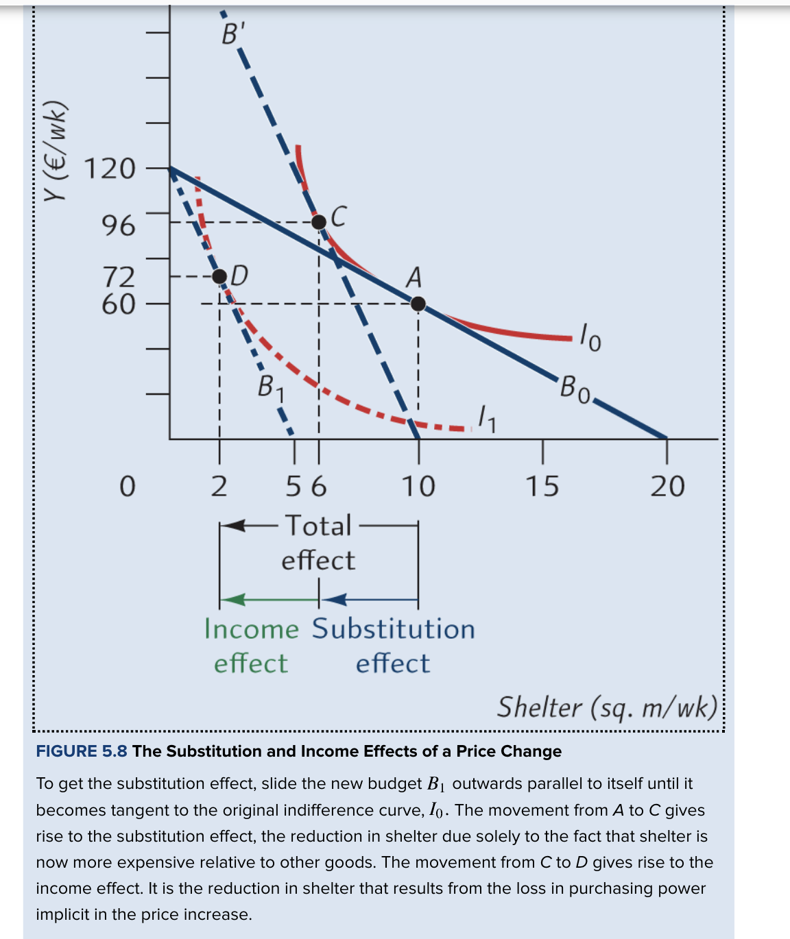
How to draw the hypothetical budget line

1. Draw the new budget line after the price change.

2. Shift it parallel outwards until it is tangent to the original indifference curve.

3. The movement from A to C is the substitution effect.

4. The movement from C to D is the income effect.

A parallel shift of the new budget line tangent to the original indifference curve.

Why is B’ hypothetical?

For a price increase for a normal good:

• It compensates for lost purchasing power to isolate the substitution effect

• Eg by increases income

Does the income effect reinforce or offset the substition effect for inferior and normal goods?

1. Inferior- offset

2. Normal- reinforce

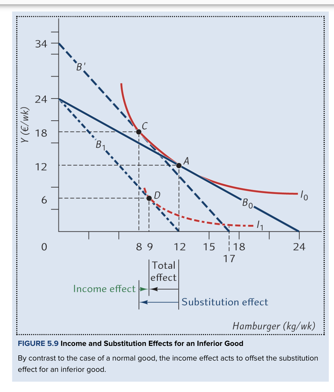
Graph for total effect for inferior good, price increase. Explain

• Consumers income is $24/week

• Y = $1/unit

• Hamburgers = $1/kg, rises to $2/kg

1. Draw BC (B0)

2. For B0, BAB = A = (12,12)

3. Price rises to $2/kg → draw B1

4. Shift outwards till tangent to B0

5. B’ shows substitution effect: A→C (8,18)

6. At B1, BAB = D = (9,6)

7. TE of price increase: reduce consumption by 3kg/week

Income effect + substitution effect oppose eachother!

• Subs effect: reduce by 4kg/week

• Income effect: increase by 1kg/week

What do Hicksian and Slutsky decompositions do?

Split the total effect iof a price change into substitution and income effects.

Hicksian vs Slutsky decomposition

Feature	Hicksian	Slutsky
Income adjusted to	Reach original indifference curve	Afford original bundle at the new prices
Holds constant	Utility	Purchasing power to buy original bundle

• Hicksian: How much income would the consumer need to reach their original indifference curve after the increase in price? (B’) (og method used)

• Slutsky: How much income would the consumer need to afford their initial bundle after the increase in price?

What does the Hicksian method hold constant?

Utility

• By keeping the consumer on the original indifference curve.

What does the Slutsky method hold constant?

The ability to afford the original bundle.

Do Hicksian and Slutsky usually give very different results?

No

• Usually similar results

Giffen good

An inferior food for which QD increases as its prices increases

What causes giffen goods?

|income effect| > |substitution effect|

• SE: P increase → QD decreases

• IE: P increase → real purchasing power falls → QD for inferior good increases

• IE stronger than SE → TE of price increase is to increase QD

Relationship betw giffen goods and inferior goods

1. All giffen goods are inferior goods

2. Not all inferior goods are giffen goods

Conditions for giffen goods

1. Strongly inferior (|IE|>|SE|)

2. Takes up large share of budget (so price increase significantly reduces PP)

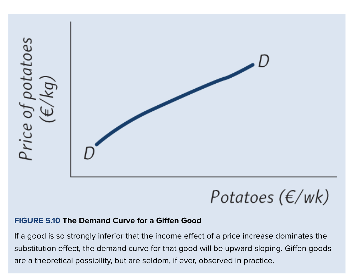
Demand curve for inferior goods vs giffen goods

1. Inferior- usually downward sloping

2. Giffen- upward sloping

Are giffen goods common or rare + why?

Rare

• Few goods meet both conditions (large share of budget + strongly inferior)

The more broadly defined a good is…

The less likely it is to be inferior

• Meat (broad) → normal

• Hamburger (specific) → inferior (+ will usually have a lot of close subs)

Example of giffen good

Potatos

• But disputed

• Poor households → potatos = huge part of diet

• Potato prices increased → households became poorer → reduced spending on expensive food (meat) to buy more potatos

Veblen good

Good a consumer may purchase at a high price to signal their wealth

Perfect complements

Goods consumed together in a fixed proportion.

Substitution effect for perfect complements

0

• So total effect = income effect

• Bc consumers buy in fixed proportion. Don’t want to substitute 1 good for another. Price of 1 increase → RPP decreases → will buy fewer complete sets

Shape of indifference curve for perfect complements

L shaped

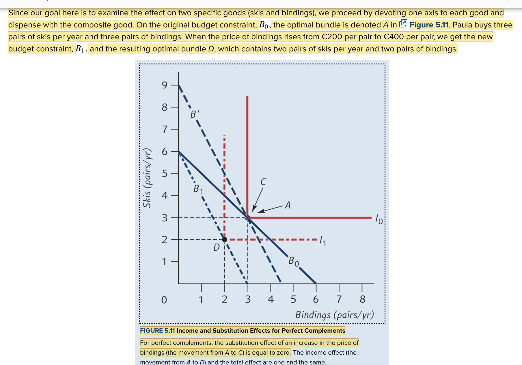
EXAMPLE 5.1 Suppose skis and bindings are perfect, one-for-one complements and Paula spends all her equipment budget of €1,200/yr on these two goods. Skis and bindings each cost €200. What will be the income and substitution effects of an increase in the price of bindings to €400 per pair?

Paula has €1,200/year. Skis and bindings initially cost €200 each.

• Initially: 3 pairs of skis + 3 pairs of bindings.

• Bindings rise to €400 each.

• New bundle: 2 pairs of skis + 2 pairs of bindings.

Effect	Change
Substitution effect	0
Income effect	1 fewer pair of skis and 1 fewer pair of bindings
Total effect	1 fewer pair of each

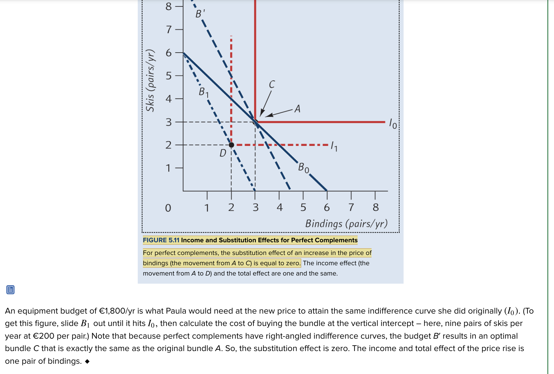
Why is the substitution effect for perfect complements 0?

Consumer can’t gain utility by changing the ratio of the goods

• So consumers maintain fixed consumption ratio

What happens when one perfect complement becomes more expensive?

Consumers buy fewer complete sets due to lower purchasing power.

Perfect substitutes

Goods consumers consider interchangeable at a constant rate

• Each good equally contributes to utility

Indifferent curves for perfect substitutes

Straight lines

How do consumers choose between perfect substitutes with different prices?

They choose the cheaper one

Why can perfect substitutes have a large substitution effect?

Consumers switch towards the relatively cheaper good

EXAMPLE 5.2 Suppose Pam considers tea and coffee to be perfect one-for-one substitutes and spends €12/wk on these two beverages. Coffee costs €1/cup, while tea costs €1.20/cup. What will be the income and substitution effects of an increase in the price of coffee to €1.50/cup?

Pam has €12/week. Coffee initially costs €1/cup; tea costs €1.20/cup.

• Initially: 12 cups of coffee, 0 cups of tea.

• Coffee rises to €1.50/cup, making tea cheaper.

• New bundle: 10 cups of tea, 0 cups of coffee.

Effect	Change
Substitution effect	Switch from 12 cups of coffee to 12 cups of tea
Income effect	0 cups
Total effect	Switch from coffee to 10 cups of tea

Perfect substitutes vs perfect complements

Feature	Perfect complements	Perfect substitutes
Indifference curves	L-shaped	Straight lines
Consumption pattern	Fixed proportion	Choose based on relative prices
Substitution effect	Zero	Can be large
Income effect	Equals total effect	Can be zero
Typical response to price rise	Buy fewer complete sets	Switch to the relatively cheaper good

What determines the substitution effect for perfect substitutes?

• How relative prices change

• + whether the preferred good switches

(idk explain this)

What determines responsiveness of consumption to price changes?

The size of the:

1. Substitution effect

2. Income effect

What determines the size of the income + substitution effect?

1. Substitution possibilities: if alternatives are available

2. Budget share: how much of a consumer’s income is spent on the good

Why is QD of salt highly insensitive to changes in price (inelastic)?

1. Few/no close subs → small substitution effect

2. Small portion of income spent → small income effect

What feature of the graph shows that salt has no close substitues?

Indifference curves are (almost) right angles

• So small substitution effect

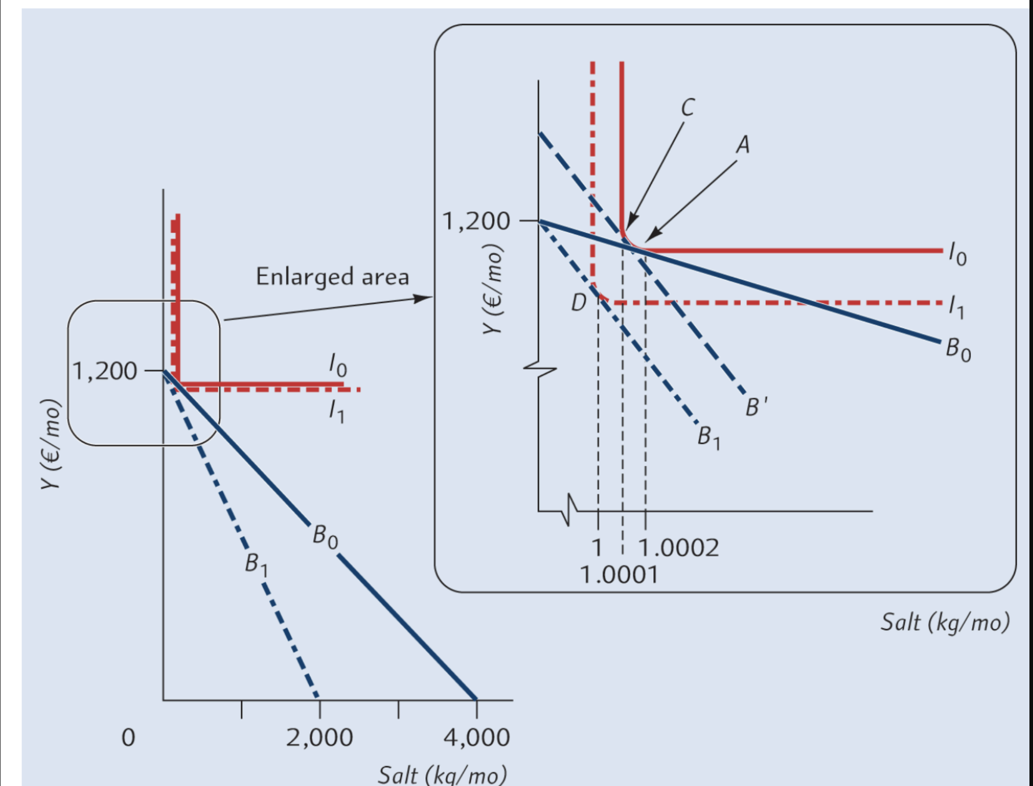
What feature of the graph shows that salt has a negligable budget share?

Cusp of ICs occur at v small quantities

• Small income effect (tiny proportion of expenditure)

When will the total effect of a price change be really small?

1. Og equilibrium bundle lies near vertical intercept of the budget constaint → causes small income effect (C→D)

• Near the pivot point of budget constaint → large rotation produces small movement

2. Indifference curves have a nearly right-angled shape → causes small sub effect (A→C)

Why is housing price sensitive?

1. Many substitution possibilities (cheaper / smaller / less central housing) → high sub effect

2. Large budget share → high income effect

Generally, what makes a good more price sensitive?

1. Many close subs → large sub effect.

2. Large share of income → large income effect

What are the two conditions for a small total effect, eg salt?

1. Og BAB is near the vertical intercept

2. Indifference curves are nearly right-angled

What feature of this graph represents that there are lots of substitution possibilities?

ICs have smooth, convex shape

• Large sub effect