PSY 3307 Lecture 8

Item analysis and correlation

item response theory, which revolutionized the way in which we think about and evaluate the performance of individual items and entire scales.

The item-total correlation is typically a Pearson correlation (r) that is calculated between a person’s score on an individual item and the total score on the entire test. On a test containing 20 items, there would be 20 item-total correlations for each of the items.

how strongly each item, or indicator, is related to the total score. If you view total score as an imperfect estimate of how much ability (or how much of a condition or characteristic) a person has of the construct being assessed, then the item-total correlation gives you an idea of how well each item measures the construct you are interested in.

Example in the textbook (page 79)

Item response theory and item Response Models

One of the fundamental differences between traditional measures of item performance, such as Cronbach’s alpha and item-total correlations and item response theory, is that traditional measures of performance are estimated from an entire sample and are treated as applicable for everyone in the sample. The item-total correlation is a sample dependent constant. An item-total correlation of 0.55 is believed to capture the degree to which an item is related to the overall amount of what the test is measuring for the entire sample but as an average summarizing the sample as a whole may not represent the extent to which items are related to the construct the test is measuring for individuals at different levels of that construct.

Item Response Models:

the fundamental challenge facing all item response models is to model the response curve linking the probability of choosing a specific option on a particular item, Pjm , and an individual’s level, θ, of the particular trait, ability or condition believed to determine whether or not an option or item is endorsed.

The most common application of IRT has been in education, where psychometricians use it for developing and refining exams, maintaining banks of items for exams and equating for the difficulties of successive versions of exams.

IRT models are often referred to as latent trait models. The term latent is used to emphasize that discrete item responses are taken to be observable manifestations of hypothesized traits, constructs, or attributes, not directly observed, but which must be inferred from the manifest responses.

Classical test theory and item response theory

Item response models acknowledge explicitly that the probability of an individual endorsing a specific item or option is an inherently stochastic process – which means that there are a whole bunch of factors that make it more or less likely that someone will choose an option but there is no certainty.

Stochastic terms and Option Characteristic Curves

In stochastic terms, we are interested in the probability of an individual endorsing option m from item j as a function of depressive severity, θ, which can be expressed as,

Pjm (θ). Pjm (θ) is a curve, that has a value between 0 and 1 (because it is a probability) and the value of Pjm (which is between 0 and 1) will vary depending on the value of θ, which is your level of depression, amount of ability, etc.

Option Characteristic Curves

Option characteristic curves correspond to graded statements, such as on the BDI or HRSD, which may be endorsed by individuals or clinicians or they may correspond to levels of a Likert scale, such as on the NEO-PI.

Option characteristic curves (OCCs) represent the probability of a specific response option being endorsed or observed at any level of the trait, ability or condition.

Option characteristic curves (OCCs)

(a) how discriminating an option is relative to other options and (b) over what range of depressive severity options discriminate among individual differences. As expected, the probability of not observing “depressed feeling states” (Option 0) decreases rapidly as depressive severity begins to increase, whereas the probability of observing “depressed feeling states indicated only on questioning” (Option 1), increases in the minimal to moderate range of depression and then decreases rapidly. In contrast, the probability of “Depressed feeling states spontaneously reported verbally” (Option 2) increases rapidly in the moderately depressed range of depressive severity but then begins to decrease as depressive severity reaches severe levels, whereas “patient reports VIRTUALLY ONLY these feeling states in his spontaneous verbal and nonverbal communications” (Option 4) only begins to be endorsed in the most severe range of depressive severity. As desired, the region in which “communicated depressed feeling states nonverbally” (Option 3) is most likely to be endorsed falls between the regions in which Option 2 and Option 4 are most likely to be endorsed.

Features of Option Characteristic Curves:

First, option characteristic curves differ with respect to the region of depressive severity in which options are most likely to be endorsed. The threshold for endorsing Option 2 is relatively low (i.e., it is rated by clinicians within a minimal to moderate range of depressive severity). The threshold at which Option 2 is rated by clinicians 40% of the time corresponds to an overall severity score of about 10 to 20, whereas the threshold at which Option 3 is rated by clinicians 40% of the time corresponds to an overall severity score of about 25.

Second, option characteristic curves differ with respect to the rate (or slope) at which the probability of being endorsed changes with increases in depressive severity. The threshold at which the option characteristic curve for Option 2 is endorsed is more discrete (i.e., steeper) than the threshold at which Option 3 is endorsed. That is, the probability of a clinician endorsing Option 2 increases faster with changes in depressive severity than the probability of endorsing Option 3. Greater slope equals greater discrimination.

Third, option characteristic curves differ with respect to how accurately response curves have been estimated. Confidence intervals for Option 0 from Item 1 (Depressed Mood) show that Option 0 is estimated more precisely than Option 4. curves are estimated more precisely in the central, denser regions of the sample than in the more extreme, less dense regions. For example, the 95 percent confidence region for Option 3 is narrower for expected total scores ranging from 10 to 20 than for the 95 percent confidence region in the 25 to 30 range.

Difficulty

Difficulty reflects the amount of a condition, trait or ability required to endorse a response. For example, Option 4 from the Depressed Mood question in Figure 1 is only endorsed at a high level of depressive severity. In this sense, difficulty is like the threshold at which an option is endorsed. The threshold at which Option 1 is first endorsed is much lower. It is often useful to have a standard point of comparison, such as the point along θ, or that namely the amount of depression, at which an option has a 0.50 chance of being endorsed. 0.50 is what is traditionally used, but it could have some other value. Whatever the value is, this value becomes the benchmark for comparison.

Discriminability

Discriminability reflects the ability of test scores on a measure to detect real differences in some ability, trait or condition. The discriminability of an option is captured by the slope of the option characteristic curve. Steeper slope means that an option is better able to detect a difference.

A 2-unit change in depressive severity from -2 to 0 corresponds to a 0.10 change in the probability (from 0 to 0.10) that the option is endorsed. However, the same 2-unit change in depressive severity from +2 to +4 corresponds to a 0.40 change in probability (from 0.50 to 0.80).

If an increase in depressive severity is not accompanied by a change in the probability of the option being endorsed, then the option is not sensitive to any change or difference. For example, a 2-unit change from -4 to -2 produces no appreciable change in the probability of the option being endorsed. In this region of depressive severity this option is in-sensitive to changes in depressive severity. It would fail to discriminate among individuals with different levels of depressive severity in the -4 to -2 region of depressive severity.

Precision

Precision refers to the extent to which you can infer how depressed a person is from the option that is endorsed.

If the person chooses Option 3, then what level of severity does the person have? Chances are it somewhere between -1 and 3 (along the x-axis). 27.9 which is the region of depressive severity that falls directly below the “peak” for Option 3.

Let’s suppose that the person chose Option 1. What level of severity does the person have? Somewhere between -2 and 0 – which is much narrower and therefore much more precise. In this way, Option 1, does a better job of telling us how depressed a person might be.

Area under the curve

Option 1: 95% certainty that the actual level of depression is in the bottom half of the curve 

Option 3: 95% certainty that the actual level of depression is in the top half of the curve 

As the curve gets steeper guessing how much depression someone has gets better 

How accurate: determining where you fall in the curve

Option 2: broad estimate of where someone falls

Option Characteristics Curves

First, the range in which most options are endorsed most frequently can be clearly identified; second, option characteristic curves change rapidly with changes in depressive severity; and third, the region in which options are most likely to be endorsed corresponds to the ordinal position implied by the weights assigned to options.

Option 3 is more likely to be endorsed than Option 4. Option 4 represents a more severe degree of depressed mood than Option 3.

All of these features—the threshold at which items are endorsed (i.e., level of depressive severity), the slope of the threshold, and the precision with which option characteristic curves are estimated—express how effective the option is as an indicator of the trait, ability or condition of interest.

Item response models for ability tests (right-wrong answers)

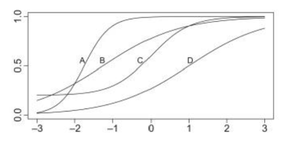
Describe the difference between the items marked A and D in terms of 

Discriminability: is the slope of the curve, it's the probability of getting the question correct. For question A it would be the probability that everyone is likely getting the question correct. Whereas for question D the probability of getting the questions correct is lower. A has better discriminability because the slope is localized in the area where the majority of the people will likely get in correct. 

Difficulty: The difficulty level of question A is a z-score of -2. And question D is 1. So the majority of the people are getting A right but some people will be able to get D right. By using the arbitrary point of 0.5 on the x-axis to get the estimated z-score. 

Precision : Which one is more precise 

95% of the area under the curve of the question D is more precise because there is less of a range (-3-3) 

95% of the area under the curve of question A is from -3-0. Higher range is less precise.