Business Stats

Data is described in 3 ways:

Tables: (freq distribution, Graphs (Bar charts, Histogram), Numerical Measures (Measures of central tendency; location, i.e perecntiles; dispersion)

Position of median

Mean of Sample Data

X bar

Mean of population Data

Meu

what do percentiles do?

Give the relative position/location of the element in the dataset

Percentile Location formula

i = percentile location, P = percentile

Element location for a percentile formula (when i isn’t an integer)

first element, found using location from i, + (difference between 2nd element - first element)* (the decimal component of i)

Q1

25th percentile

Q3

75th percentile

IQR

Q3-Q1

Upper Limit of boxplot

Q3+1.5*IQR

Lower limit of boxplot

Q1- 1.5*IQR

Any data beyond the limits are:

Outliers

Measure of Dispersion + Ex of it

Tell us the spread of the data (do data values remain consistent or do they change a lot) Ex: STD DEV

If range is low:

Values are relatively close and there’s less fluctuation in data

STD Dev (def + formula)

Tells us how far away from the mean data values are + square root of variance

STD Dev of sample formula

sqr root of:

STD Dev of population formula

Sqr Root of:

The higher the std dev:

further away values are from the mean

random experiment

Outcome of which can’t be predicted with certainty

Random variable (denoted by?)

All possible values based on the random experiment; X

Probability

Discrete Random variables

Values obtained by Counting (ex: # of siblings)

Continous Random Variable

Values obtained by measuring (ex: height)

Characteristics of Discrete Probability Distribution

• RV will be discrete

• Prob value is given by formula

Conditions for Binomial Prob Distribution

• RV will be discrete

• IITF

IITF

Identical trials, Independent Trials, Two outcomes for each trial (success or failure), Fixed probabilities for both out outcomes in every trial

Binomial Formula

Types of Continous Probability Distributions

Uniform, Normal

Properties for a graph of a continous probability distribution

Shape is the same as a histogram, Probability = Area under graph, total area under a graph = 1

Properties of a graph of a uniform distribution

Shape is rectangular, probability = area under graph = 1

What’s the probability that flight time is exactly 136.111 mins?

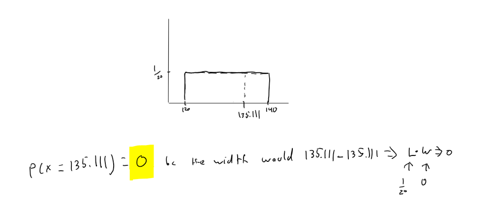
Why is P(120 < x < 130) = P (120≤ x ≤ 130) true?

Bc the lines P(X=120) and P(X=130) are 0

Properties of Normal Distribution

Bell shape, Probability = Area = 1, Mean = Median, Empirical Rule

Empirical Rule

68% of area within 1 STD DEV, 95% of area within 2 STD DEVs, 99% of area within 3 STD DEVs

Z-Score formula

Z-Score values show the area of the Z-Score to the…?

Left

Inferential Statistics

Understanding a population using a sample

Random Sampling

Every population unit is given an equal chance to be part of the sample

Point Estimator + examples

Estimate is a specific point

Mean of Sample Means = ?

Mean of Population (i.e Meu)

Std Dev of Sample Means = ?

Shape of the distribution of a sample mean (x-bar) is normal when:

• n (i.e. sample size) is greater or equal to 30

• Population is normally distributed

For finding probabilities of a normal distribution of sample means, the z-score formula is:

Proportion

(number of observations with a characteristic) / (total number of observations)

P-hat

sample proportio

P

Population Proportion

Mean of Sample Proportions = __

Population Proportion (i.e P)

STD DEV of Sample Proportion

The shape of the distribution of sample proportions is normal when?

• np > 5

AND

• n(1-p) >5

n= sample size

p= population proportion

The z-score formula for normally distributed sample proportions =