PSYC 300A - Unit 2

Explain bivariate data

Involves two variables (X & Y)

• Often two datapoints from the same thing (e.g., person)

• But can be two things related by something (such as date)

• Correlation: Method to describe the relationship between two variables

  • Varies from -1 to 1 (e.g., r = 0.30)

• Regression: Predicting the values of one variable from another variable

  • Includes a slope and an intercept

What is the difference between correlation and regression?

• Correlation is just seeing if there’s a relationship between the two variables

• Whereas regression is trying to predict one variable from the other variable

How can we visualize bivariate data from a scatterplot

Describing relationships

• From a Scatterplot:

  • Direction: Positive or negative

  • Strength: Weak, moderate, strong (subjective; based on visual)

  • Shape: Linear or curvilinear

How can we measure bivariate data from a correlation coefficient

Describing relationships

• From a Correlation Coefficient:

  • Direction: Positive or negative

  • Magnitude: Size (objective) (r = -0.64)

  • Strength: Weak, moderate, strong (based on r value)

  • Shape: Linear or curvilinear

How to computing correlation

Steps for dealing with Bivariate Data:

1. Plot data

2. Apply descriptive statistics (mean, SD) to each variable

3. Apply descriptive statistics to the joint variables

4. Compute correlation coefficient

What is Pearson r

Pearson r: Degree to which two variables covary

• Standardized measure of correlation

  • Means we can compare it across studies

  • Could even compare it across things that are unrelated

• r = Cov/(SDx)(SDy)

How can we describe bivariate data in a formal report

For our five participants, there was a strong, negative, linear relationship, r = -0.64, between participant shoe size (Ȳ = 7.00, SD = 2.00) and 1km run time (x̅ = 3.00, SD = 1.10). As shoe size increased, run time decreased.

What are factors that influence Pearson r

1. Relationship is real and strong/weak

2. Sampling error

3. Unmeasured third variable

4. Heterogenous sample

5. Truncated ranges

6. Non-linear relationship

7. Heteroscedasticity

Explain sampling error

Sampling error: discrepancy between sample statistics and population parameter

• Each sample had inherent variability from the population

• Central tendency and variability then may differ across samples

• Each sample may increase or decrease r by chance

• May increase or decrease r

Explain unmeasured third variable

Unmeasured Third Variable:

• Two things can be related because of some other factor that we didn’t track in our study

  • Eg. crime is correlated with ice cream sales because both increase with better weather

• Mediation and moderation tests can be used to test for third variable influences (these are not covered in this course)

• May increase or decrease r

Explain heterogenous sample

Heterogenous Sample: When your sample includes multiple sub-samples

• Can decrease r if sub-samples behave differently

• Can increase r by chance if subsamples line up into a correlation

• May increase or decrease r

Explain truncated range

Truncated Range: When data are collected from a restricted range of the full scale, the resulting scores may provide incomplete or misleading information about the true relationship across the entire range

• Most often reduces r

• But in some cases can increase r by chance

• May increase or decrease r

Explain non-linear relationships

Non-Linear Relationships: Correlations may not be linear

• Treating a non-linear relationship as linear can decrease r

• Treating a linear relationship as non-linear can also decrease r

• There exists non-linear tests (this is part of regression)

• Decreases r

Explain heteroscedasticity

Heteroscedasticity: Variability changes across our range

• Remember, COV/(SDx)(SDy), so increases in variability (SD) will reduce r

• Heteroscedasticity can be caused by a skew in one or both of our variables

• Decreases r

Explain sample size

• There is an incorrect assumption that the larger the sample size, the larger the correlation

• In fact, sample size does not have any direct impact on correlations

• It will, however, have an on whether we decide the correlation is significant

• Does not affect r

Explain when we use other scales and correlation

Explain regression conceptually

Regression allows us to predict a variable’s score (e.g. a y-value) from a score on another variable (e.g., an x-value)

• A mathematically defined line that best represents the bivariate relationship

Explain slope

How much one variable changes when another variable increases by 1

Explain y-intercept

How much of one variable do you have in the absence of the other

Explain error in regression

Although we can come up with a very good prediction of Y from X, variability in our data makes it unlikely that we will find a perfect prediction

Compare explained variability and unexplained variability

Explained Variability: How close our predictions are from the actual value

• In other words, how well have we predicted one variable form the other

Unexplained Variability: How far our predictions are from the actual value

• In other words, how poorly we predicted one variable from the other

What is the regression line denoted as

The regression line is denoted a Y’ and X’

• Y’ = ay + by(X)

  • Y’ = Predicted y-values from the regression line

  • ay = Y-intercept

    • How much of Y when there is an absence of X

    • The y-value when X = 0

    • A constant in the equation that shifts the regression up or down

  • by = Slope

    • How much Y-scores change across X-scores

    • How much Y changes for a single increase in X

    • A coefficient in the equation that changes the steepness of the relationship

• X’ = ax + bx(Y)

  • X’ = predicted X-values from the regression line

  • ax = X-intercept

    • How much of X when there is an absence of Y

    • The x-value when Y = 0

    • A constant in the equation that shifts the regression left or right

  • bx = slope

    • How much X-scores change across Y-scores

    • How much X changes for a single increase in Y

What are the steps for computing regression?

1. Plot your data

2. Determine mean and SD for X and Y

3. Compute Pearson r

4. Compute the slops (by & bx)

5. Compute the intercepts (ay & ax)

6. Define the regression lines (Y’ & X’)

7. Plot the regression lines

8. Compute the standard error

How to determine mean and SD for X and Y

How to compute Pearson r

r = Cov/(SDx)(SDy)

How to compute the slopes (b_y & b_x)

• When predicting Y from X

  • For Y’ = ay + by(X)

  • by = r(SDy/SDx)

• When predicting X from Y

  • For: X’ ax + bx(Y)

  • bx = r(SDx/SDy)

How to compute the intercepts (a_y & a_x)

• When predicting Y from X

  • For: Y’ = ay + by(X)

  • ay = y̅ - by (x̅)

    • This is where the regression line hits the Y-axis

• When predicting X from Y

  • For: X’ = ax + bx(Y)

  • ax = x̅- bx (y̅)

    • This is where the regression line hits the X-axis

How to define the regression lines (Y’ & X’)

Defining the regression line is to write out the equation with the computed coefficients (slope and intercept)

• Y’ = a y + by(X)

  • ay & by are coefficients

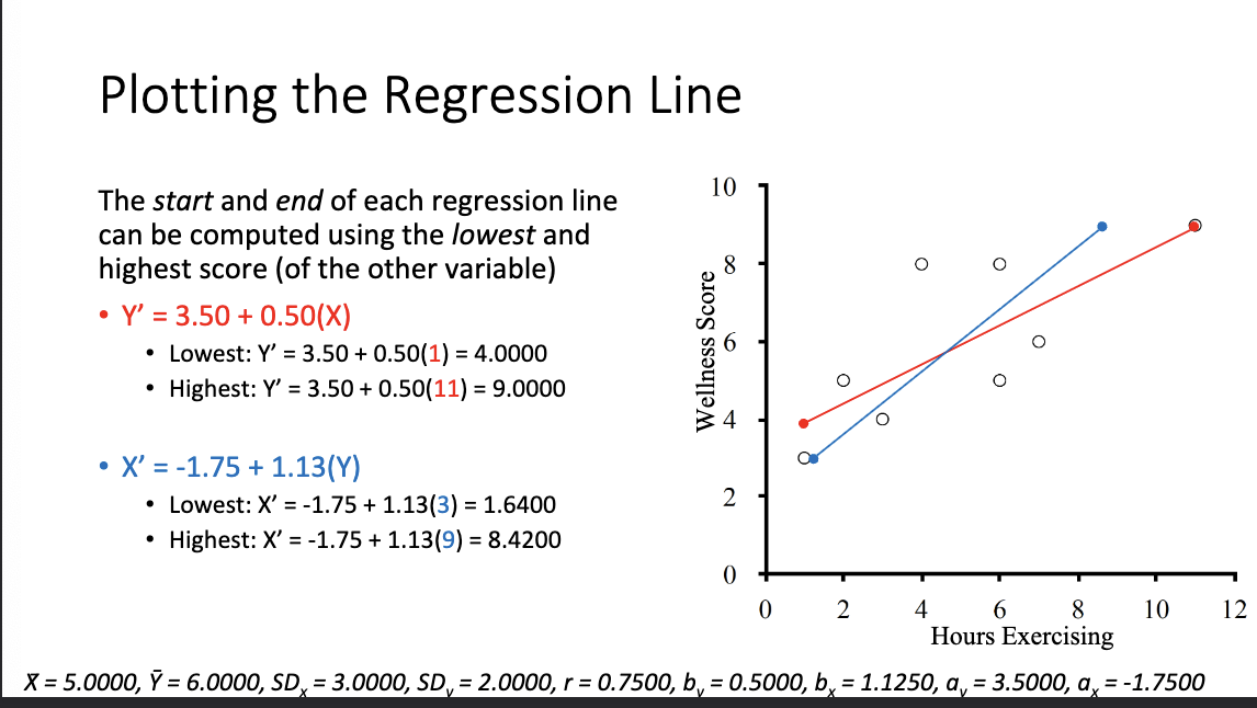
• Y’ = 3.50 + 0.50(X) ← this is the defined regression line

• X’ = ax + bx(Y)

  • a x & b x are coefficients

• X’ = -1.75 + 1.13(Y) ← this is the defined regression line

How to plot the regression lines

Plotting a regression line means we need to know different points on that regression line

1. We already know the intercepts

2. The regression lines also converge where the mean of X and Y meet

3. We can also calculate any point on the regression lines using the equation just defined

• Y’ = 3.50 + 0.50(X)

  • For X = 4: Y’ = 3.5000 + 0.5000(4) = 5.50

4. The start and end of each regression line can be computed using the lowest and highest score (of the other variable)

• Important note: The regression lines DO NOT go past the data

  • Because we can only predict scores within our observed data

  • Interpolation, not extrapolation

    • Interpolation: Estimating unknown values within known data points

    • Extrapolation: Estimating unknown values outside of known data points

Regression and correlation

If r = 0 then slopes (by & bx) = 0

• Regression line is parallel to the axes

• The regression lines then simply becomes the mean of Y and X

• a y = y̅, a x = x̅

• Y’ = a y + byX

• Y’ = a y + 0X

• Y’ = a y = y̅

• Y’ = y̅

• As r increases, the slope increases

  • The two regression lines converge towards becoming the same

    • At r = ±1, they completely overlap

Explain standard error of the regression line

Residuals: The deviation each score is from the predicted value of the regression line

• Y-Y’ , X-X’

• SDy’ = SDy√1-r²

• SDx’ = SDx√1-r²

What is notation for total variability?

• Xo

• Y-Ȳ

• 1

• SSt

• ∑(Y-Ȳ)²

What is notation for explained variability?

• Xt

• Y’-Ȳ

• r²

• SSr

• ∑(Y’-Ȳ)²

What is notation for unexplained variability

• Xe

• Y-Y’

• 1-r²

• SSe

• ∑(Y-Y’)²

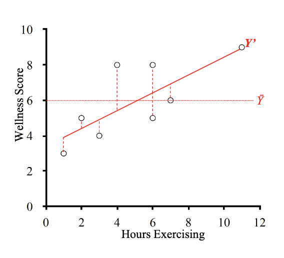
What is explained variability in regression?

How much error is reduced because we are taking into account the correlation

• We are not asking if a regression is good or not but instead asking if it’s better than the mean

• It’s better if the scores are closer to the regression line than to the mean

• When r = 0, SDy = SDx

  • Everything is unexplained variability

  • Different scores of X predict same Y-values (i.e. the mean of Y)

• When r = ±1, SDy’ = 0

  • Everything is explained variability

  • Prediction is more accurate because we are accounting for two sources

What is r and r²

• r: Standardized measure of association between X and Y

• r²: Proportion (or percent when x100) of variability accounted for in Y by variability in X

How to write formal report for regression

We investigated the relationship between hours of exercise (x̅ = 5.00, SDx = 3.00) and a person’s wellness (y̅ = 6.00, SDy = 2.00) in eight individuals, see Figure 1. There was a strong, positive, linear relationshiip between hours of exercise and wellness (r = 0.75, by = 0.50, ay = 3.50, SDy’ = 1.32, bx = 1.13, ax = -1.75, SDx = 1.98), which explained 56% of variability in our data. In summary, increased hours of exercise was associated with increased wellness.