ch 10 assumptions of the pearson r and alternative measures of correlation

During the era of Enlightenment, the philosopher _____ wrote the book Candide. 

Voltaire

intro to the chapter

• During the era of Enlightenment, the philosopher Voltaire wrote the book Candide. The main characters in the book are Candide, an idealistic young man, and his sidekick, a philosopher named Pangloss (said to be patterned after the real philosopher Leibnitz, the co-discoverer of calculus). The two men travel the world in an effort to understand and better it.

• Pangloss, in particular, is full of high flown theories that tend to justify the unjustifiable, excuse the inexcusable, and lead to disaster whenever an effort is made to apply them. After several years of nearly unrelenting troubles brought on by their own efforts, Candide and Pangloss decide that the secret of successful living is simplicity. They settle down on a small country place and become subsistence farmers. They have one cardinal rule of conduct: no discussion of philosophy is allowed. However, one day as they are blissfully hoeing the potatoes, a weighty philosophical question occurs to Pangloss. He says "You know, I wonder if..." Without pausing or looking up, Candide interrupts, saying "Shut up and hoe the potatoes." In this book we have tried very hard to stick closely to the hoeing in the interest of simplicity.

• But there are some issues of a theoretical or even philosophical nature with which we must occasionally deal. These issues must be considered in order to most effectively use our statistical methods and to appreciate how they function as tools in the broader human endeavor of science.

Platonic idealism

The ancient Greek philosopher Plato believed that there existed two distinct related worlds. One was the sensory world - what we might call the world of ever experence or the material world - where we perceive the things around us through our senses. We see tables, mountains, animals and the other objects in the world a us.

The other world was the ideal world, a non-material world of ideas. The two worlds are related in that the things in the sensory world are imperfect copies of the ideas in the ideal world. For example, we see tables in the everyday or sensory world.

The idea of "tableness" exists in the ideal world. My dining table is an imperfect of the idea of tableness (my dining table has some scuffs and scratches in the varnish and a gouge on one leg).

• Plato developed this idea in his allegory of the cave. He said that we live our lives like prisoners in a cave, tied up in such a way that we can only see the wall in front of us. The only source of light is a fire behind us. The real action of the world takes place between the fire and us. Thus, what we see are the shadows of that reality cast on the wall in front of us. The shadow images derive from and do resemble the real action taking place behind us, but they are dark, shimmering, imperfect copies of it.

• By now, if you are a "normal" person, you are wondering why we are so far off the track of statistics. This philosophy stuff seems to border on the downright wacky.

• The example of "tableness" seems strained and artificial. It is unclear how any of this relates to statistics. You might even think that the authors, after a shaky start, have finally lost it altogether.

• Perhaps we should look at some other examples. Consider the definition of a line. A line is perfectly straight; it has no width; and it extends forever. It we attempt to draw a line (as in Figure 10-1) on a piece of paper, a blackboard, or any other surface, it will not be possible to make it perfectly straight, without width, and infinitely long. We might, however, make it fairly straight, very thin, and somewhat long. Similarly, a point is said to have position, but not extension. That is, it does not take up any space.

• Again, any attempt to draw a point (as in Figure 10-1) will fall short, because it will actually occupy some space.

• Clearly, "lineness and "pointness" exist only in the perfect world of ideas. Yet, our admittedly imperfect applications of them in the everyday, sensory world are extraordinarily useful when we do things like survey land for a highway or navigate a ship at sea. In fact, the field of mathematics is filled with these sorts of imperfect applications of perfect ideas.

• Infinite sets of numbers, instantaneous slopes of curved lines, and shapes sliced into pieces so thin that there are an infinite number of them are all ideas that cannot be perfectly produced in the everyday world. But applications of these ideas are very useful in creating the comfortable and prosperous everyday world we inhabit today.

Platonic idealism:

The ancient Greek philosopher ____ believed that there existed two distinct related worlds.

plato

What are the two distict related worlds plato believed in

sensory world

ideal world

Platonic idealism:

What is the sensory world

 what we might call the world of everyday experience or the material world - where we perceive the things around us through our senses. We see tables, mountains, animals and the other objects in the world a us. 

Platonic idealism:

What is the ideal world?

 a non-material world of ideas. The two worlds are related in that the things in the sensory world are imperfect copies of the ideas in the ideal world. For example, we see tables in the everyday or sensory world.

The idea of "tableness" exists in the ideal world. My dining table is an imperfect of the idea of tableness (my dining table has some scuffs and scratches in the varnish and a gouge on one leg).

Plato developed this idea in his allegory of the cave. 

• He said that we live our lives like prisoners in a cave, tied up in such a way that we can only see the wall in front of us. The only source of light is a fire behind us. The real action of the world takes place between the fire and us. Thus, ….

• what we see are the shadows of that reality cast on the wall in front of us. The shadow images derive from and do resemble the real action taking place behind us, but they are dark, shimmering, imperfect copies of it.

By now, if you are a "normal" person, you are wondering why we are so far off the track of statistics. This philosophy stuff seems to border on the downright wacky.

• The example of "tableness" seems strained and artificial. It is unclear how any of this relates to statistics. You might even think that the authors, after a shaky start, have finally lost it altogether.

• Perhaps we should look at some other examples:

consider the defintion of a line

• Consider the definition of a line. A line is perfectly straight; it has no width; and it extends forever. It we attempt to draw a line (as in Figure 10-1) on a piece of paper, a blackboard, or any other surface, it will not be possible to make it perfectly straight, without width, and infinitely long. We might, however, make it fairly straight, very thin, and somewhat long. Similarly, a point is said to have position, but not extension. That is, it does not take up any space.

• Again, any attempt to draw a point (as in Figure 10-1) will fall short, because it will actually occupy some space.

• Clearly, "lineness and "pointness" exist only in the perfect world of ideas. Yet, our admittedly imperfect applications of them in the everyday, sensory world are extraordinarily useful when we do things like survey land for a highway or navigate a ship at sea. In fact, the field of mathematics is filled with these sorts of imperfect applications of perfect ideas.

• • Infinite sets of numbers, instantaneous slopes of curved lines, and shapes sliced into pieces so thin that there are an infinite number of them are all ideas that cannot be perfectly produced in the everyday world. But applications of these ideas are very useful in creating the comfortable and prosperous everyday world we inhabit today.

describe a line

perfectly straight; it has no width and it extends forever

a point is said to have postion but not…

extension, that is it doesnt take up any space

• again any attempt to draw a point (as in the figue 10-1) will fall short, because it will actually occupy some space.

Clearly, "lineness and "pointness" exist only in the perfect world of ideas. yet..

• Yet, our admittedly imperfect applications of them in the everyday, sensory world are extraordinarily useful when we do things like survey land for a highway or navigate a ship at sea. In fact, the field of mathematics is filled with these sorts of imperfect applications of perfect ideas.

Infinite sets of numbers, instantaneous slopes of curved lines, and shapes sliced into pieces so thin that there are an infinite number of them are all ideas that cannot be perfectly produced in the everyday world. but..

• But applications of these ideas are very useful in creating the comfortable and prosperous everyday world we inhabit today.

SCIENTIFIC THEORY AND IDEALIZATION

• Modern scientific theories work largely by this process of idealization. They consist of a set of ideas that create a "model" that represents some process in the natural world. We may never find the ideas exactly duplicated in the everyday world.

• However, if the theory is a useful one, the duplication is close enough that successful predictions can be made from the model and an improved understanding of the material world can be achieved. For example, Isaac Newton's First Law of Motion states that an object in motion tends to remain in motion. Did you ever see an object in motion that actually remained in motion? All the objects that we have ever seen have tended to stop —- usually pretty quickly. Even the motion of the planets is slowing perceptibly 

• Nevertheless, the principles of newtons physicals have served us very well. They allow us to predict the positions  of the planets years in advance, to hit a target with artillery from miles away, and to send a space vehicle to the moon or mars 

SCIENTIFIC THEORY AND IDEALIZATION

• Modern scientific theories work largely by this process of idealization

  • they consist of ..

• a set of ideas that create a "model" that represents some process in the natural world. We may never find the ideas exactly duplicated in the everyday world.

  • • However, if the theory is a useful one, the duplication is close enough that successful predictions can be made from the model and an improved understanding of the material world can be achieved.

    • For example, Isaac Newton's First Law of Motion states that an object in motion tends to remain in motion. Did you ever see an object in motion that actually remained in motion? All the objects that we have ever seen have tended to stop —- usually pretty quickly. Even the motion of the planets is slowing perceptibly 

      • Nevertheless, the principles of newtons physicals have served us very well. They allow us to predict the positions  of the planets years in advance, to hit a target with artillery from miles away, and to send a space vehicle to the moon or mars 

STATISTICAL MODELS:

• When we work with statistical methods we also employ this process of idealization and modeling. We have a set of ideas that we use to describe some process or thing. These ideas create a model that helps us to better conceive of, understand, and work with that thing.

  • For example, earlier in this book we worked with percentages under the normal curve for tests of intellectual ability. In this case we used the normal curve as a model for the nature of human intellectual performance, and we assumed that our test scores are ot an appropriate level of measurement (the levels of measurement discussed in Chapter One are models of measurement that form the basis for this sort of modeling).

• Almost certainly our models are not perfect. The distribution of human intellectual performance is probably not a perfect normal distribution. Likewise, our measurement of human intellectual performance is probably not a truly interval level of measurement. But we come close enough to fulfilling these idealized assumptions that our work is useful in both a practical and a theoretical sense.

• To summarize this discussion we can say that behind any theoretical model or prediction system is a set of assumptions. These assumptions will probably not be met perfectly and the model will probably not perfectly describe the material world.

• However, it is important that we know what our assumptions are, that we have a carefully considered idea of how accurate these assumptions are, and that we take this into account when deciding to apply our statistical model.

When we work with statistical methods we also employ this process of idealization and modeling. We have a set of ideas that we use to describe some process or thing. These ideas create…

• a model that helps us to better conceive of, understand, and work with that thing.

  • For example, earlier in this book we worked with percentages under the normal curve for tests of intellectual ability. In this case we used the normal curve as a model for the nature of human intellectual performance, and we assumed that our test scores are ot an appropriate level of measurement (the levels of measurement discussed in Chapter One are models of measurement that form the basis for this sort of modeling).

statistical models:

• Almost certainly our models are not perfect. The distribution of human intellectual performance is probably not….

a perfect normal distribution.

• Likewise, our measurement of human intellectual performance is probably not a truly interval level of measurement.

  • But we come close enough to fulfilling these idealized assumptions that our work is useful in both a practical and a theoretical sense.

staitistical models, summary

• To summarize this discussion we can say that behind any theoretical model or prediction system is a set of assumptions. These assumptions will probably not be met perfectly and the model will probably not perfectly describe the material world.

  • However, it is important that we know what our assumptions are, that we have a carefully considered idea of how accurate these assumptions are, and that we take this into account when deciding to apply our statistical model.

APPLICATION TO CORRELATION:

• The Pearson product moment correlation to on coefficient, like any other statistical procedure, makes certain assumptions about the data being examined 

• The accuracy of everything we have said in the last three chapters (about strength of the relationship, ability to make predictions, and forecasting prediction error) depends on the degree to which the scores fit the model created by these assumptions. While the assumptions will rarely be met perfectly, more extreme violations of the assumptions will produce more serious errors in the conclusions we draw from the results of our calculations.

  • For this reason we must always be aware of the assumptions behind our procedures and be sensitive to the appropriateness of our data for the statistical method we use.

The Pearson product moment correlation coefficient, like any other statistical procedure, does what

makes certain assumptions about the data being examined 

ASSUMPTIONS OF THE PEARSON R:

• Four assumptions underlie. The Pearson r. These assumptions are listed and explained below 

1. Assumption 1: both variables to be correlated are continuous variables.

2. Assumption 2:Both variables are of interval level of measurement or ratio level of measurement.

3. Assumption 3: The relationship between the two variables is linear.

4. Assumption 4: The relationship between the variables is characterized by the property of homoscedasticity

Assumption 1 of the pearson r

• both variables to be correlated are continuous variables.

• A continuous variable has an infinite number of possible values arranged in infinitely small steps. An example of a continuous variable is weight (measured in pounds).

• There are an infinite number of weights a person might have and there is no minimum difference between weights that could not be further reduced. One person might weigh 155 pounds and another might weigh 154 pounds. A third person could weigh 154.9 pounds or 154.97 pounds. For any score we might choose, however close to 155, there can always be another even closer to 155. Thus, there is no limit on closeness between two scores. This is in contrast to the other major type of variable - a discrete variable.

• A discrete variable usually (but not always) has a finite set of possible values that are arranged in a step-like manner (always), so that we must go all the way from one value to the next value as if each value were a step on a ladder. An example of a discrete variable would be the score obtained when tossing a die (singular of dice). The lowest score we could get would be a 1. The next lowest score would be a 2. We could not get a 1.2 or 1.78, as would be possible with a continuous variable; and there are only six possible outcomes, 1 through 6. A dichotomous variable is a special kind of discrete variable. A dichotomous variable has only two possible outcomes.

  • For example, the answer to a question could be scored as either correct or incorrect. Or a switch could be either on or off

assumtion 1 of the pearson r: Both variables to be correlated are continuous variables

• A continuous variable has what…

• an infinite number of possible values arranged in infinitely small steps. An example of a continuous variable is weight (measured in pounds).

  • There are an infinite number of weights a person might have and there is no minimum difference between weights that could not be further reduced. One person might weigh 155 pounds and another might weigh 154 pounds. A third person could weigh 154.9 pounds or 154.97 pounds. For any score we might choose, however close to 155, there can always be another even closer to 155. Thus, there is no limit on closeness between two scores. This is in contrast to the other major type of variable - a discrete variable.

What is discrete variable?

• usually (but not always) has a finite set of possible values that are arranged in a step-like manner (always), so that we must go all the way from one value to the next value as if each value were a step on a ladder.

  • An example of a discrete variable would be the score obtained when tossing a die (singular of dice). The lowest score we could get would be a 1. The next lowest score would be a 2. We could not get a 1.2 or 1.78, as would be possible with a continuous variable; and there are only six possible outcomes, 1 through 6.

    • A dichotomous variable is a special kind of discrete variable. A dichotomous variable has only two possible outcomes. For example, the answer to a question could be scored as either correct or incorrect. Or a switch could be either on or off

What is a dichotomous variable

• a special kind of discrete variable.

• A dichotomous variable has only two possible outcomes.

  • For example, the answer to a question could be scored as either correct or incorrect. Or a switch could be either on or off

What is …. assumption 2 of the pearson r

• Both variables are of interval level of measurement or ratio level of measurement.

• Recall from Chapter One that in an interval scale of measurement (and in a ratio scale of measurement) equal sized intervals between scores represent equal sized differences in the variable being measured. That is, the 10 degree difference between 35 degrees Fahrenheit and 45 degrees Fahrenheit represents the same difference in temperature as the 10 degree difference between 85 degrees Fahrenheit nd 95 degrees Fahrenheit.

• What is… Assumption 3: of the pearson  r

• The relationship between the two variables is linear.

• This assumption states that the relationship between the two variables is best described by a straight line (rather than a curved line). The scattergram of a linear relationship between two variables shown in Figure 10-2 illustrates a case in which Assumption 3 is met.

  • In contrast, Figure 10-3 shows the scattergram of a non-linear relationship between variables - a case in which Assumption 3 is not met.

• The Pearson r measures the prediction efficiency of the best straight line that can be fit to the data. A Pearson r computed on the data in Figure 10-3 would yield a correlation coefficient of just about zero. This would lead to the erroneous conclusion that there is no relationship between the two variables. Actually, however, we can see that there is a quite strong relationship between the variables; it is just not a linear relationship.

The pearson r measures what

the prediction efficiency of the best straight line that can be fit to the data.

Assumption 4 of the pearson r

• The relationship between the variables is characterized by the property of homoscedasticity.

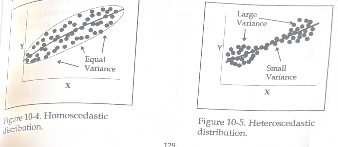
• In a homoscedastic relationship the variance around the regression line remains the same throughout the range of the two variables. This characteristic is what produces the smooth elliptical shape of a scattergram, as shown in Figure 10-4.

  • On the other hand, the scattergram of a heteroscedastic relationship may have irregular lumps or bulges along its length, such as is shown in Figure 10-5.

• How do you know if assumptions have been seriously violated? Although there is no guaranteed, cut-and-dried method, it is usually possible to determine whether or not the assumptions of the Pearson r have been seriously violated. Visual inspection of the scattergram will usually reveal a serious departure from linearity or homoscedasticity.

  • And a careful consideration of the way the scores were generated will usually tell us something about how well we have met the assumptions of continuously scored variables and interval or ratio level measurement of the variables.

    
    

• What if assumptions have been seriously violated? If our variables do seriously violate the assumptions of the Pearson r, then it is clearly inappropriate to employ this procedure. However, it is not the end of the world. There are other measures of correlation that require different assumptions and/or less stringent assumptions. We can usually find one of these other measures of correlation that is appropriate for our data. As an example, in the next section we will consider one of these alternate forms of correlation 

assumption 4 of the pearson r:The relationship between the variables is characterized by the property of homoscedasticity.

what is a homoscedastic relationship?

• the variance around the regression line remains the same throughout the range of the two variables.

  • This characteristic is what produces the smooth elliptical shape of a scattergram, as shown in Figure 10-4.

  • On the other hand, the scattergram of a heteroscedastic relationship may have irregular lumps or bulges along its length, such as is shown in Figure 10-5.

assumtion 4 of the pearson r: The relationship between the variables is characterized by the property of homoscedasticity.

• How do you know if assumptions have been seriously violated? 

Although there is no guaranteed, cut-and-dried method, it is usually possible to determine whether or not the assumptions of the Pearson r have been seriously violated. Visual inspection of the scattergram will usually reveal a serious departure from linearity or homoscedasticity.

And a careful consideration of the way the scores were generated will usually tell us something about how well we have met the assumptions of continuously scored variables and interval or ratio level measurement of the variables.

assumtion 4 of the pearson r: The relationship between the variables is characterized by the property of homoscedasticity.

What if assumptions have been seriously violated?

• if our variables do seriously violate the assumptions of the Pearson r, then it is clearly inappropriate to employ this procedure.

• However, it is not the end of the world. There are other measures of correlation that require different assumptions and/or less stringent assumptions. We can usually find one of these other measures of correlation that is appropriate for our data. As an example, in the next section we will consider one of these alternate forms of correlation 

SPEARMANS RHO:

• Spearmans rho is made for situations in which our data are in the form of ranks (Ranking represents an ordinal level of measurement; thus, the Pearson r assumption of interval or ratio levels of measurement is not met).

  • Informally, Spearman's tho is sometimes called a rank-order correlation coefficient.

• The computation of Spearman's rho is based on the squared differences between ranks for each pair of observations on our two variables. Since this squared difference is the only thing that must be calculated from the data, computation of Spearman's rho is much simpler than the computation of the Pearson r.

• As an example, suppose we conducted a study attempting to assess the effectiveness of the interview as a selection technique for hiring new employees for our company. In particular, we wish to determine the reliability of our interview process.

  • That is, to what extent do the interviews produce consistent results? (An interview cannot yield accurate results if it cannot produce consistent results.) We ask two interviewers to independently interview five applicants for the same job and to rank the applicants on their perceived suitability for the job. These rankings are given in Table 10-1.

• As we mentioned previously, the computation of Spearman's rho is based on the sum of squared differences between ranks on the two variables (in this case the two interviewers) for each subject (in this case each applicant). If the differences tend to be small, the correlation will be high. If the differences tend to be large, the correlation will be low.

Informally, Spearman's tho is sometimes called..

a rank-order correlation coefficient

The computation of Spearman's rho is based on

• the squared differences between ranks for each pair of observations on our two variables.

  • Since this squared difference is the only thing that must be calculated from the data, computation of Spearman's rho is much simpler than the computation of the Pearson r.

Spearman’s rho example:

• As an example, suppose we conducted a study attempting to assess the effectiveness of the interview as a selection technique for hiring new employees for our company. In particular, we wish to determine the reliability of our interview process.

• That is, to what extent do the interviews produce consistent results? (An interview cannot yield accurate results if it cannot produce consistent results.) We ask two interviewers to independently interview five applicants for the same job and to rank the applicants on their perceived suitability for the job. These rankings are given in Table 10-1.

Applicant	Rank assigned by interviewer #1	Rank assigned by interviewer #2
1	2	3
2	4	1
3	5	4
4	1	2
5	3	5

table 10-1

• As we mentioned previously, the computation of Spearman's rho is based on the sum of squared differences between ranks on the two variables (in this case the two interviewers) for each subject (in this case each applicant). If the differences tend to be small, the correlation will be high. If the differences tend to be large, the correlation will be low.

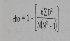
• The formula for spermans rho is 

formula for spearmans rho

• 10-2 shows the necessary quantities and the calculations for rho.

• where D is the difference in ranks on the two variables for one subject, and N is the number of subjects or cases in the study.

Spearmans rho example continued:

• Now we can use this formula to calculate rho for our interviewing study. 

• Table 10-2 Ranks Assigned to Five Job Applicants by Two Interviewers: Calculation of rho

Applicant	Rank interviewer #1	Rank interviewer #2	D difference	D(squared) (difference)squared
1	2	3	-1	1
2	4	1	3	9
3	5	4	1	1
4	1	2	-1	1
5	3	5	-2	4
				(summation symbol )D(squared)= 16

Spearmans rho example continued:

(click on image to see the problem worked out)

• Based on the value of our correlation coefficient, rho= .20, we would conclude that our interviewers were not in very close agreement on their rankings of the job applicants. Perhaps we should change our interviewing process

Additional issues regarding correlation:

• In this section we discuss two issues that frequently are associated with errors in  the interpretation of correlations.

  • The first issue arises when we have several correlation coefficients (for example, from several different studies) and we want to calculate an average correlation. In this case we must take into account the fact that correlations do not constitute an interval scale of measurement; we cannot simply ad the correlations and divide by the number of correlations.

  • The second issue stems from the fact that if one thing causes something else, then the two things must be correlat However, if two things are correlated, it does not necessarily mean that one causes other. Each of these issues is discussed in more detail below.

• Averaging correlations. As we saw in Chapter Nine (see Table 9-6), the error eliminated (measured by the index of forecasting efficiency) as correlations increase grows faster when correlations are large than when they are small. That is, the difference in explanatory power between correlations of .30 and .40 is much less than that between correlations of .80 and .90.

• Because of this, it is inappropriate to average correlations in their raw form.

  • Fortunately, the great statistician Ronald Fisher created a transformation (now commonly called Fisher's z - not to be confused with the standard score or z-score that we introduced in Chapter 5) that gets around this problem. Appendix D contains the table for the Fisher's z transformation. Note that in Appendix D each value of r has an associated value of z, and the values of z increase slowly when r is low and increase more rapidly when r is large.

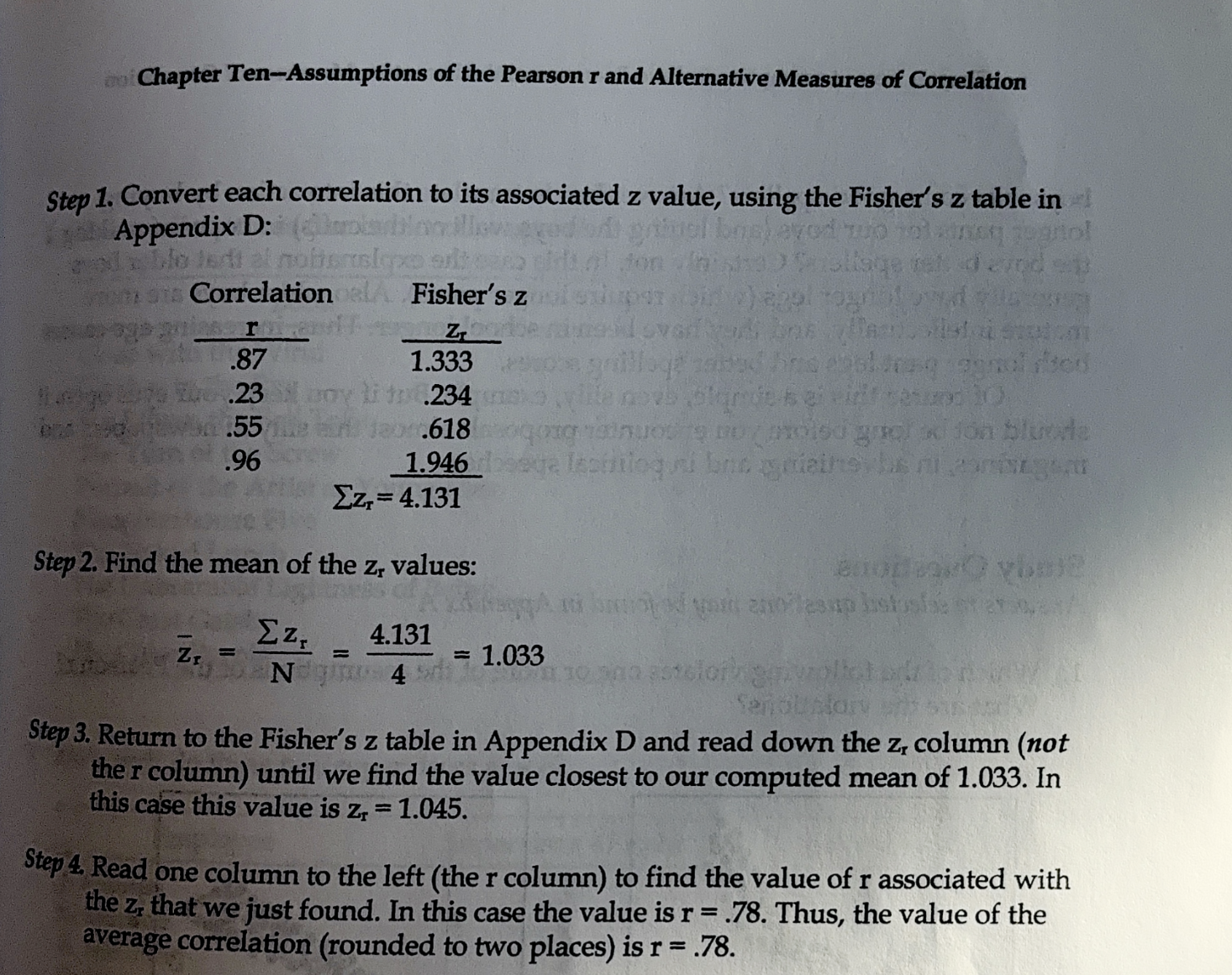
• As an example, suppose that we have created a test to predict the widget makin ability of applicants for jobs in the widget industry. Furthermore, we have done a stuc of the test's ability to predict widget output of workers at four widget plants. The correlations are .87, .27, .55, and .96. We wish to report the average correlation for the study. As we stated earlier, it is not appropriate to simply add the four raw correlations and then divide by four to get an average correlation of .66. 

  • Instead, the proper way to find the average correlation is to use Fisher's z transformation in Appendix D according to the following step-by-step procedure:

• Correlation and causation

  • . It is widely and erroneously believed that if two things are correlated, one must cause the other. Newspapers and popular magazines frequently print articles that make this (incorrect) leap from correlation to causation. In these cases, it is also amusing that the authors of these articles appear to be certain that they can identify which variable is the cause and which variable is the effect.

  • As an example, suppose we know that having taken Latin in high school is correlated with good grades in college. The error is to conclude that taking Latin in high school causes good grades in college. And this error is compounded when we then suggest that all students should be required to take Latin in high school, because this will make them all good students.

  • If you learn nothing else from this book than that correlation does not imply causation, then you have probably gotten your money's worth. At best, a causal relationship is very difficult to establish; it requires many controlled, experimental studies (like those discussed later in this book), rather than a single correlational study.

  • For the purpose of illustration, consider this laughably simple example. Suppose that we go to a grade school, measure the length of the pant legs for all the boys, and give all boys a spelling test. We would almost certainly find a high correlation between pant leg length and spelling test score. Are we to conclude that long pant legs cause boys to become good spellers? Are we then to translate this into action by buying longer pants for our boys (and letting the boys walk on the cuffs) in hopes of making the boys better spellers? Certainly not. In this case the explanation is that older boys generally have longer legs (which require longer pants). Also, older boys are more mature intellectually, and they have been in school longer. Thus, increasing age causes both longer pant legs and better spelling scores.

  • Of course this is a simple even silly example but if you keep your eyes open it should not be long before you encounter proposals almost this silly in the news and magazines in ads and political speeches 

What are two issues that frequently are associated with errors in  the interpretation of correlations.

• The first issue arises when we have several correlation coefficients (for example, from several different studies) and we want to calculate an average correlation. In this case we must take into account the fact that correlations do not constitute an interval scale of measurement; we cannot simply ad the correlations and divide by the number of correlations.

• The second issue stems fr the fact that if one thing causes something else, then the two things must be correlation

• However, if two things are correlated, it does not necessarily mean that one causes other. Each of these issues is discussed in more detail below.

if two things are correlated, it does not necessarily mean that..

one causes other

issues associated with errors in interpretation correlation: Averaging correlations.

As we saw in Chapter Nine (see Table 9-6), the erro eliminated (measured by the index of forecasting efficiency) as correlations increase grows faster when..

• correlations are large than when they are small. That is, the difference in explanatory power between correlations of .30 and .40 is much less than that between correlations of .80 and .90. Because of this, it is inappropriate to average correlations in their raw form.

  • Fortunately, the great statistician Ronald Fisher created a transformation (now commonly called Fisher's z - not to be confused with the standard score or z-score that we introduced in Chapter 5) that gets around this problem. Appendix D contains the table for the Fisher's z transformation. Note that in Appendix D each value of r has an associated value of z, and the values of z increase slowly when r is low and increase more rapidly when r is large.

  • As an example, suppose that we have created a test to predict the widget making ability of applicants for jobs in the widget industry. Furthermore, we have done a stuc of the test's ability to predict widget output of workers at four widget plants. The correlations are .87, .27, .55, and .96. We wish to report the average correlation for the study. As we stated earlier, it is not appropriate to simply add the four raw correlatic and then divide by four to get an average correlation of .66. 

  • Instead, the proper way to find the average correlation is to use Fisher's z transformation in Appendix D according to the following step-by-step procedure: 

Who created a transformation (now commonly called Fisher's z - not to be confused with the standard score or z-score that we introduced in Chapter 5) that gets around this problem. 

ronald fisher

issues associated weith errors in interpretation of correlation: Correlation and causation

• . It is widely and erroneously believed that if two things are correlated, one must cause the other. Newspapers and popular magazines frequently print articles that make this (incorrect) leap from correlation to causation. In these cases, it is also amusing that the authors of these articles appear to be certain that they can identify which variable is the cause and which variable is the effect.

  • As an example, suppose we know that having taken Latin in high school is correlated with good grades in college. The error is to conclude that taking Latin in high school causes good grades in college. And this error is compounded when we then suggest that all students should be required to take Latin in high school, because this will make them all good students.

  • If you learn nothing else from this book than that correlation does not imply causation, then you have probably gotten your money's worth. At best, a causal relationship is very difficult to establish; it requires many controlled, experimental studies (like those discussed later in this book), rather than a single correlational study.

  • For the purpose of illustration, consider this laughably simple example. Suppose that we go to a grade school, measure the length of the pant legs for all the boys, and give all boys a spelling test. We would almost certainly find a high correlation between pant leg length and spelling test score. Are we to conclude that long pant legs cause boys to become good spellers? Are we then to translate this into action by buying longer pants for our boys (and letting the boys walk on the cuffs) in hopes of making the boys better spellers? Certainly not. In this case the explanation is that older boys generally have longer legs (which require longer pants). Also, older boys are more mature intellectually, and they have been in school longer. Thus, increasing age causes both longer pant legs and better spelling scores.

  • Of course this is a simple even silly example but if you keep your eyes open it should not be long before you encounter proposals almost this silly in the news and magazines in ads and political speeches 

Examples of issues with interpreting correlation and casuation

• As an example, suppose we know that having taken Latin in high school is correlated with good grades in college. The error is to conclude that taking Latin in high school causes good grades in college. And this error is compounded when we then suggest that all students should be required to take Latin in high school, because this will make them all good students.

• If you learn nothing else from this book than that correlation does not imply causation, then you have probably gotten your money's worth. At best, a causal relationship is very difficult to establish; it requires many controlled, experimental studies (like those discussed later in this book), rather than a single correlational study.

• For the purpose of illustration, consider this laughably simple example. Suppose that we go to a grade school, measure the length of the pant legs for all the boys, and give all boys a spelling test. We would almost certainly find a high correlation between pant leg length and spelling test score. Are we to conclude that long pant legs cause boys to become good spellers? Are we then to translate this into action by buying longer pants for our boys (and letting the boys walk on the cuffs) in hopes of making the boys better spellers? Certainly not. In this case the explanation is that older boys generally have longer legs (which require longer pants). Also, older boys are more mature intellectually, and they have been in school longer. Thus, increasing age causes both longer pant legs and better spelling scores.

• Of course this is a simple even silly example but if you keep your eyes open it should not be long before you encounter proposals almost this silly in the news and magazines in ads and political speeches