Mod 5

Boolean Logic

A type of logic that deals with variables that can only have the values of true or false.

Apostrophe (')

A symbol used in Excel to indicate that the contents of a cell should be interpreted as text.

Quotations ("")

The use of quotations in Excel to indicate that the contents of a cell should be interpreted as text and not as a formula.

Concatenation Operator (&)

An operator in Excel used to combine text and cell references by using the & symbol.
=”your total is “&D5&” plase pay in 30 days.”

Concatenate function

=CONCATENATE(B1,B5)
It combines the selected cells together

TEXT function

A function in Excel used to convert a number to text in a specific format.
=TEXT(D5, “$0.00”) converts the number to dollar format

UPPER function

A function in Excel used to convert text to uppercase.

LEFT function

A function in Excel used to extract a specified number of characters from the beginning of a text from the left.

RIGHT function

A function in Excel used to extract a specified number of characters from the end of a text.

MID function

A function in Excel used to extract a specified number of characters from the middle of a text. Obtain text, starting from specific character and extracting a number of letters.
=MID(C9,10,10)
starting from character number 10 and give me 10 chararters

FIND function

A function in Excel used to find the position of a character or text within another text.
=LEFT(C3,FIND(C13,”@”)-1)
This will obtain the text before the @

Multiple Worksheets

The use of multiple worksheets within a single Excel workbook. Use ! then the cell reference (B2), then the operation (+)
=Sheet1!B2+Shee2!B2

Relative Cell References

Cell references in Excel that change when a formula is copied to another cell.

Absolute Cell References

Cell references in Excel that do not change when a formula is copied to another cell.

Boolean Values

The values true or false that can be assigned to a Boolean variable.

Equals (=) Operator

An operator in Boolean logic that compares two values and produces a Boolean result.

NOT Operator

A Boolean operator that negates the value of a variable. If the variable is true, NOT(X) is false, and if the variable is false, NOT(X) is true.

AND Operator

A Boolean operator that returns true only if both variables being evaluated are true. If either variable is false, the result of AND(X,Y) is false.

OR Operator

A Boolean operator that returns true if at least one of the variables being evaluated is true. If both variables are false, the result of OR(X,Y) is false.

XOR

A Boolean operator that returns true if exactly one of the variables being evaluated is true. If both variables are true or both variables are false, the result of XOR(X,Y) is false.

Inclusive OR

An OR operator that allows for the possibility of both variables being true. If either variable is true or both variables are true, the result of OR(X,Y) is true.

Excel always uses inclusive OR.

Exclusive OR

An OR operator that does not allow for the possibility of both variables being true. If either variable is true, but not both, the result of XOR(X,Y) is true.

Greater than (x>y)

A comparison operator that returns true if the value on the left is greater than the value on the right.

Less than (x<y)

A comparison operator that returns “true” if the value on the left is less than the value on the right.

Less than or equal to (

A comparison operator that returns “true” if the value on the left is less than or equal to the value on the right.

Equal to (=)

A comparison operator that returns “true” if the value on the left is equal to the value on the right.

IF

A Boolean function that evaluates a logical test and returns one value if the test is true, and another value if the test is false.
=IF(condition , value_if_true, value_if_false)

ISBLANK function

A function that checks if a cell is blank. Can be used as a condition in IF function.

=B3&” “& IF(ISBLACNK(C3), ,C3&” “) &D3

&→shows text
Overall, shows that if the middle name is blank & true , then text will not show, but if this is false, then text will include the last name and a space by &” “

ISERROR function

A function that checks if a value is an error.

IFERROR function

A function that returns a specified value if a formula results in an error.

=IFERROR(AVERAGE(E2:E4),0)

If there is an error in the result, proceed with 0, othersie, produce the value calculated.

COUNTIF function

A function that counts the number of cells that meet a specified condition.

=COUNTIF(range, criteria)

=COUNTIF(E4:E103,”>1000”)

Count the number of orders between this range, if they are greater than 1000.

SUMIF

=SUMIF(range, criteria, [sum_range])

The criteria is used in the range, so you can search a value in the range. The sum_range references the values in the range and sums the values that match the criteria.

AVERAGEIF function

A function that calculates the average of cells that meet a specified condition.

=AVERAGEIF(RANGE, CRITERIA, [AVERAGE RANGE])

If this range has this criteria, then average the numbers within this range.

COUNTBLANK

A function that counts the number of blank cells in a specified range.

=COUNTBLANK(A7:F7)

COUNTIFS

A function that counts the number of cells that meet multiple criteria. E.g make sure that the counted cells are from Alberta but also above 1000.

=COUNTIFS(criteria_range1, criteria1,criteria_range2,criteria2...etc) 

criteria_range1: Required. The first range in which to evaluate the associated criteria.

criteria1: Required. The criteria in the form of a number, expression, cell reference, or text that define which cells will be counted. For example, criteria can be expressed as 32, ">32", B4, "apples", or "32".

criteria_range2, criteria2, ...: Optional. Additional ranges and their associated criteria. Up to 127 range/criteria pairs are allowed.

EXAMPLE: describes the correct usage of COUNTIFS for counting the number of Excel cells within the range E3 to E9 which displays a value that is less than 100 but greater than 50. 

ANS:

criteria_range1: $E$3:$E$9

criteria1: ">50"

criteria_range2: $E$3:$E$9

criteria2: "<100"

VLOOKUP

A function that looks up a value in a table and returns a corresponding value from a specified column.

=VLOOKUP(lookup_value, table_array, col_index_num,[range_lookup])

lookup value - uses this value for reference

table array - uses this range to search for the lookup value

col_index_num - the column you want the results from

[range_lookup] - Boolean TRUE or FALSE. True for an approximate match or false for an exact match of the lookup value.

What is the significance of setting the match parameter in a VLOOKUP function to be True?

The exact match or the closest value in the table that is still less than the value (if there is no exact match) will be returned

When using VLOOKUP, entering the lettering case (uppercase/lowercase) will affect your results.

I.e., There is a difference between =VLOOKUP("apple",....) and =VLOOKUP("APPLE",....).

False

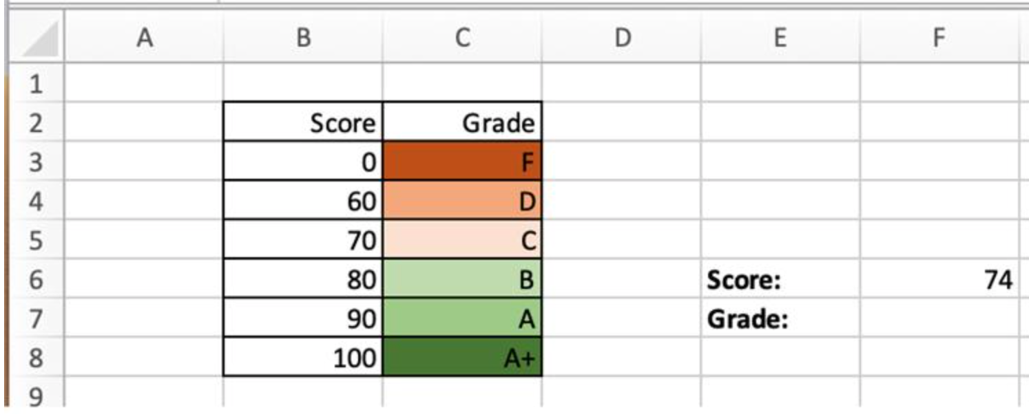
What is the most appropriate formula to input in cell F7 to produce the grade that corresponds to the score in F6?

=VLOOKUP(F6,B3:C8,2,TRUE)

AVERAGEIF

A function that calculates the average of cells that meet a specified criteria.

AVERAGEIF(range, criteria, [average_range])

SUMIF

A function that calculates the sum of cells that meet a specified criteria.

SUMIF(range, criteria, [sum_range])

IFERROR

A function that returns a specified value if a formula results in an error.

IFERROR(value, value_if_error)

value   The argument that is checked for an error.

value_if_error   The value to return if the formula evaluates to an error. The following error types are evaluated: #N/A, #VALUE!, #REF!, #DIV/0!, #NUM!, #NAME?, or #NULL!.

HLOOKUP

A function similar to VLOOKUP, but it looks up values across rows instead of columns.

HLOOKUP(lookup_value, table_array, row_index_num, [range_lookup])

• Lookup_value    Required. The value to be found in the first row of the table. Lookup_value can be a value, a reference, or a text string.

• Table_array    Required. A table of information in which data is looked up. Use a reference to a range or a range name.

  • The values in the first row of table_array can be text, numbers, or logical values.

  • If range_lookup is TRUE, the values in the first row of table_array must be placed in ascending order: ...-2, -1, 0, 1, 2,... , A-Z, FALSE, TRUE; otherwise, HLOOKUP may not give the correct value. If range_lookup is FALSE, table_array does not need to be sorted.