Regression Analysis Exam Unit 1

What is the multiple regression model?

What are all the components of the MLR model?

• y is the dependent variable that is a random variable with mean of the betas and variance sigma² and is normally distributed

• the x’s next to the betas are independent variables that can be quantitative, qualitative or higher order terms

• E(y) = … is the determonisitc component (“the average” part of the model)

• $\beta_i$ = the contribution of predictor $x_i$, holding the other variables constant.

What is the experimental region?

range of observed combinations of x’s

What are the steps of MLR?

1. Collect sample data

2. Hypothesize the model form via EDA (Unit 1.2: check each predictor vs. response; Unit 3: check relationships between predictors)

3. Estimate parameters via least squares (Unit 1)

4. Specify the error distribution & estimate variance (Unit 1)

5. Evaluate model utility (Unit 1)

6. Check model assumptions, adjust if needed (Unit 3)

7. Use the model for prediction or estimation (Unit 1)

What do you do in Step 1 of MLR?

Collect Data

• Make sure the source is reliable

Data Organization:

• Are the data organized for MLR?

  • Each row contains information about one observation(experimental unit) including all of the explanatory predictors and response

  • R Functions to know

    • Head - gives first 6 rows of data

• Make sure response variable is suitable for regression

How do we make sure response variable is suitable for regression?

• Create a histogram of response variable

• Should be continuous (or discrete over a wide range of value with a few outliners)

• Should not be recorded over time

• Sometimes useful if response variable is unimodal + symmetric but not required

What is step 2 of MLR?

• hypothesize model form through EDA

How can we create a more linear relationship?

• We can attempt to transform explanatory or response variable to create a more linear relationship

• If we transform response variables to improve relationships for one explanatory variable, we must have that transformation for every variable. Sometimes this is not worth it

• We can have some explanatory variables transformed and some left untransformed

• We don’t need to perform the same transformation to the explanatory variables and/or response

• Sometimes a “transformation” includes fitting a “curvilinear” term, in which case we retain the linear and higher order terms(x and x^2)

What is our goal of EDA?

• is to identity the univariable relationship between each explanatory variable and the response

• We do this by creating scatter plots and correlations for each variable then attempting any necessary transformation to find the most linear relationships that best fit all of the data

• After classifying these, we select variables with the strongest relationships

What does step 3 of MLR entail?

Estimate Model Paramteres(fit the model using R)

• Use the estimates for each parameter to make the prediction equation

• hat(weighted total) = -8.42+ 1.658sqrt(gdp) +0.03788(total athletes) -.001952(distance) + 0.000 Distance squared

How do we interpret coeffcients?

Ex: For a billion dollar increase in the square root of GDP, the predicted weighted medal total is expected to increase by 1.658, given the other explanatory variables are held constant

• The coefficients for the linear and curvilinear components of distance are not practical to interpret individually

What is step 4?

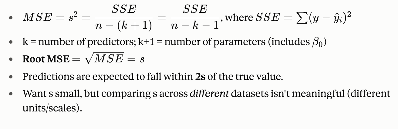
Specify the distribution of the errors and find the estimate of variance

• Estimate of sd is sqrt(mse)

• Estimate of sd^2 is MSE

• Approximately 95% of our predictions will be withing 2 * sd medals of the actual weighted medal total. Whether this is good depends great;y on goals of prediction here

• purpose of this is to quantify how much “noise” surrounds model.

What is MSE?

a statistical metric that measures the average squared difference between a model's predicted values and the actual observed values

What does it mean by estimate of σ² is MSE?

MSE (Mean Squared Error) is your point estimate of the true error variance.

What does it mean by estimate of σ is √MSE?

Since variance is in squared units (which is hard to interpret — "squared medals" doesn't mean anything), you take the square root to get back to the original units. This is called Root MSE (also written as $s$). This is the number that actually shows up in your R output as "Residual standard error."

What does it mean by Approximately 95% of predictions within 2×sd?

Empirical rule applied here. Since errors are assumed normal, about 95% of a normal distribution falls within 2 standard deviations of the mean. Applied to your model, that means: about 95% of your predicted weighted medal totals should land within ±2×(Root MSE) of the country's actual weighted medal total.

What is Step 5?

Evaluating the utility of the model

How do we evaluate the utility of our model?

By performing the global f test

What does the Global F Test do and how do we do it?

answers one question: "Is this model, as a whole, worth anything?" by testing all of the beta parameters simultaneously

The Hypotheses $H_0: \beta_1=\beta_2=\dots=\beta_k=0 \qquad H_a: \text{at least one }\beta_i\neq0$

Notice $\beta_0$ (the intercept) is not included in this test — you're only testing whether the predictors matter, not the intercept itself.

• H₀ true would mean: none of your explanatory variables help predict y at all — the model is useless.

• Hₐ true means: at least one predictor is doing something useful — but the test doesn't tell you which one(s). That's the job of the individual t-tests that come after.

Distribution of test statistic F with (k, n-k-1)

• P value

  • Reject if less than alpha 

  • Fail to reject if more than alpha

• Conclusion

  • Reject H0: model is adequate. At least one beta is not equal to 0 —> move on to individual t-tests on the predictors

  • Fail to reject: Model is inadequate —> none of the betas are significantly different from 0 so stop here or try a different set of predictors

What does k and n mean in DF?

n is the sample size

k is the number of predictors so the number of explanatory variables in your model not counting Beta 0(the intercept)

K + 1 = total number of parameters including beta -

n-k-1: error/residual degrees of freedom. represents hoe much independent information is left over after model has used up some of the data just to estimate its own parameters

If we find that the model is adqeuate, what test do we do next?

T-test because it looks at individual parameters

How does the t test work?

Answers the question: Given that all the other predictors are already sitting in the model, does this one specific predictor still pull its weight? —> testing one beta at a time, not the whole model at once

Hypotheses $H_0:\beta_i=0 \qquad H_a:\beta_i\neq0$

• $H_0$: this predictor doesn't contribute to predicting y (once the other variables are accounted for)

• $H_a$: this predictor does contribute

Distribution of test statistic: n-k-1

P value

Decision : Reject $H_0$ if p-value < α (or equivalently, $|t| > t_{\alpha/2}$). Fail to reject if p-value > α.

• Reject → the variable is significant → keep it in the model

• Fail to reject → not significant → remove it from the model

Co

Why shouldn’t you test everything in t test and how do we know which parameters to test?

• you’ll get an inflated type 1 error if you test everythig

• higher-order / curvilinear terms are almost always worth testing

• Variables your research question is actually about.

• Anything you’re specifically deciding to drop

Why do we refit the model and what does it do?

• Refitting model can change significance of other variables and will always change to beta estimates. 

• In the example, the estimates changed slightly because the term we removed was not significant

• and then you get your updated prediction equation (y hat)

What is the further assesment component?

• interpret root mse

• interpret adjusted r²

What is adjusted r²

• Measures the relationship between the 2 variables 

• We use this because we’re adjusting number of predictors compared to number of observations

• Ex Writeup: After accounting for number of predictors and observations, 87.3% of variation in weighted medal count is explained with the sqrt of gdp, total athletes, and distance

What is the relationship between the results from the t- tests and confidence intervals?

• When the pvalue doesn’t contain 0, the p value is more significant, it is statistica;;y different from o (pvalue<alpha)

• Opposite true as well

• If alpha is .05 and confidence level was 0.95 would interval for distance contain 0?

  • Yes, because p-value won’t change

What is the Step 7?

Use the Model for estimation or prediction

Estimation vs Prediction

Prediction: used when we want to predict a single observation from its set of predictors. We are using prediction here because we are making a guess about the outcome a single country. Prediction is trying to guess an indidual y

• Compute via predict function for an observation in the data table

Estimation:  used when we want to make a guess about the average of several observations that all have the same set of predictors

• average value of the response variable for a given X

How do the confidence intervals differ between estimation and prediction?

estimation has a narrower confidence interval with no extra MSE term. The difference is purely about which uncettainty(individual r average) which is why the interval widths differ but the fitted value doesn’t

• prediction interval is always wider than a confidence interval for the same predictor values, because predicting one individual has more uncertainty than estimating an average.

How do we write the interpretation for confidence intervals?

We are ___% confident that the ___ is between lwr and upr given _____

What is least squares regression?

a statistical method used to find the line of best fit for a set of data points by minimizing the sum of the squared differences (residuals) between actual and predicted values

What are the assumptions behind least squares?

For any fixed combination of $x_1,...,x_k$, the error term ε:

1. Has a normal probability distribution

2. Is centered at 0 (mean 0)

3. Has variance $\sigma^2$ (constant across all x combinations)

4. All errors are statistically independent

**linear" regression means $E(y)$ is a linear function of the parameters, not that each x must have a straight-line relationship with y.

What is a first order model?

All predictors are quantitative with purely linear contributions (no squared/higher-order terms).

Independent variables also can't be functions of each other (e.g., you can't have both x and 2x as separate predictors).

What is Least Squares Estimation with multiple predictors?

Still minimizing $SSE=\sum(y-\hat y_i)^2$,

but now across k parameters simultaneously — done via calculus (partial derivatives set to 0) and matrix algebra (beyond this course; software does it).

Each $\hat\beta_i$ is a random variable — it changes from sample to sample even from the same population. Least squares prediction equation:

$$\hat y_i = \hat\beta_0+\hat\beta_1x_1+\hat\beta_2x_2+\dots+\hat\beta_kx_k$$

What does it mean by σ² is also the variance of y

Parameter vs Estimator

Parameters = unknown, fixed, true for the population. Estimators = random variables that vary sample to sample.

What is quadratic regression

Linear regression" ≠ straight-line relationship — it means the β's combine linearly. So x and y can have a polynomial relationship. Class focuses on quadratic terms

What is the second order model

$$y=\beta_0+\beta_1x+\beta_2x^2+\epsilon$$

• $\beta_1$ is no longer a slope — it's a shift parameter.

• $\beta_0$ = y-intercept of the curve; $\beta_2$ = rate of curvature.

• Only test the significance of the higher-order term via t-test.

• Parent/child rule: if the quadratic (child, x²) term is significant, you must keep the linear (parent, x) term regardless of whether x alone tests significant.

What is p-th order polynomial?

$y=\beta_0+\beta_1x+\beta_2x^2+\dots+\beta_px^p+\epsilon$.

Individual parameter interpretations get too messy to bother with. Only test the highest-order term's significance; keep all lower-order terms regardless

What is the goal of global f test?

Goal = is the whole model adequate? Tests all β's at once (vs. testing individually). Compares explained vs. unexplained variation. Reject H₀ → model adequate (at least one β ≠ 0). Fail to reject → model not adequate. Caveat: "adequate" ≠ "good" — it's just the minimum bar.

We use ______ for MLR assessment because ______

adjusted r²; it penalizes unnecessary predictors

Adding any predictor pushes R² ____

up

What are the 2 goals of MLR?

predict the response for one particular subject, given its predictors, or (2) estimate the average response for a group of subjects that all share the same predictors.

y vs E(y) vs y-hat

y — the actual, observed response (random variable): full model with the error term epsilon included

• use this when writing hypothesized model

E(y) — the deterministic component (expected/average value); no eposion here

• represents true average value of y and use when goal is estimation

• A range of plausible values for the true average value of y

ŷ (y-hat) — the fitted/predicted value (from your sample)

• uses estimated coefficients (beta hars are computed through the least squares from the actual sample) no e because y hat is a single calculated prediction not a random variable with its own term

• Use this when: you've actually fit the model in R and are plugging in real numbers — this is Step 3 onward. It's your best single-number guess, whether you're using it for prediction or estimation

  • whether you intend to use your model for prediction OR estimation, you end up with the same prediction equation