12. Econ History: Interwar

After 1914: the short twentieth century

A century of conflict
• 1914–1945: the 'Second Thirty Years' War' (Churchill)
• 1917–1949: the 'European Civil War' (Nolte)
• 1947–1989: the Cold War
A century of calamities
• Global wars, global revolutions, global economic crises … and a global pandemic
A century of disintegration
• Deglobalisation: the 'globalisation backlash' of 1914–1945
• Decolonisation

Modern economic growth by Kuznets

'Modern economic growth' (Kuznets 1966): the 'epochal innovation' is the spreading application of science to production and social organisation
-Defining features
• Sustained rise in per capita product: roughly 15–30% per decade
• Faster growth of population and consumption; rising saving and investment ratios
• Structural change: output and consumption shift from agriculture to
manufacturing and services
• Rising international flows of goods, services and factors, but neither constant nor irreversible
First globalisation (c. 1860–1913) → globalisation backlash (1914–1945) → slow re-integration after 1945 → 'second globalisation' (1990s)
• Labour mobility never returned to pre-1914 levels
-Diffusion: England → Belgium, France, Switzerland, Rhineland, US → Prussia, Scandinavia → parts of Russia, central and southern Europe, Canada, Argentina, Oceania
-Japan: the only robust case outside European settlement before 1914

four phases of modern economics growth, 1870-1998

1870–1913:
• fast growth driven by globalisation and technological progress
• divergence between the West and the rest
1913–1950:
• world wars and the Great Depression
• slow growth in Europe and Asia
• new global powers: the US and the Soviet Union
1950–1973:
• the 'golden age' of economic growth
Post-1973:
• slowdown in the West
• rise of the East (e.g. Japan
World GDP per capita grew about 1.5% a year on average over 1870–1998

The Great War, 1914-1918: a watershed

A global armed conflict
• Fought mostly on European soil, but extended to the colonies
• Larger than any previous war in size, scope and destruction
End of the 'long' nineteenth century
• A watershed in modern history, with economic, social, political and
even cultural repercussions
Economic consequences
• Human casualties
• Disruption of world trade
• Crisis of global finance
• Peace settlements: redrawn borders, war reparations
• Dissolution of 4 empires 1917–19 (Russia, Prussia, Austro Hungaria, Ottoman) → many new nation-states

Military outcomes:

-The victors: Allied Powers
• United Kingdom, France, Russia (until March 1918), Italy (from 1915), United States (from 1917), … and many others
-The defeated: Central Powers
• Germany, Austria-Hungary, Ottoman Empire (Turkey), Bulgaria (from 1915)
-Outside the war: neutrals, e.g. Sweden, Switzerland, Netherlands, Denmark, Norway, Spain

The human cost of the war

Russia: the largest absolute losses (c. 3.3 million dead)
• Germany: the largest military death toll (2.05 million)
• France: the heaviest relative loss (4.3% of the population)
• Italy: a large civilian toll (589,000), 3.5% of the population
• United States: marginal losses (0.13%); it entered late and
fought far from home
• The losses fell overwhelmingly on Europe, part of why Western Europe's growth fell behind the US

The 1918-1920 influenza pandemic

The 'Spanish' flu
• Influenza pandemic caused by the H1N1 influenza A virus
• Up to 500 million infected worldwide, in three waves (1918–1920)
• Total mortality: estimates range from 30 to 100 million
A global pandemic (always named after someone else)
• Europe: the 'Spanish' flu; West Africa: the 'Brazilian' flu; Brazil: the 'German' flu
• Spain: the 'Naples soldier'
The role of the war
• Contagion spread by Allied armies and navies; carried into Europe (Brest, France) by US troops
• Wartime censorship limited information and the policy response
• But mass mobilisation had increased state capacity

Did the war make the flu deadlier

• Solid lines show the group averages.
• Average mortality was, if anything, higher among neutrals than among belligerents, but the bands overlap: no clear difference
• Large variation within each group: Mexico (c. 21) and Spain (c. 12) vs Denmark (c. 4); Hungary, Italy and Portugal (c. 10–13) vs Russia, Austria and Germany (c. 2.5–4)
• So the war may have spread the virus, but taking part in it does not
predict where mortality was highest

The flu’s death toll was concentrated in Asia

• By far the largest tolls were in Asia: Indian Empire, China and Dutch East Indies, each in the millions
• Substantial tolls in sub-Saharan Africa (French West and Equatorial Africa, Belgian Congo, South Africa) and the Americas (US, Mexico, Brazil)
• Europe's absolute toll was small by comparison
• These are absolute deaths, not rates, so large populations produce large circles (compare the per-capita rates on the previous slide).

stylised facts about the interwar economy

1. The slowdown was worldwide, but it hit regions very differently
2. The overall slowdown combined fairly satisfactory growth in the 1920s with dismal performance in the 1930s
3. International trade declined in real terms, out of line with output: the ‘globalisation backlash'
4. High and structural unemployment was the shocking new phenomenon
5. Labour productivity grew faster than in 1890–1913, especially in the 1920s
Plus: growth differed by war participation and by exit from gold

A pause in modern economic growth

Per capita growth slowed in 1913–50 in every region except the Soviet Union
• Western Europe was hit hardest, because two global conflicts were fought on European soil
• Between the wars (1921–38) Europe outgrew the US (2.0 vs 0.8): a strong 1920s and a milder 1930s
• The 1930s were dismal almost everywhere (US –1.3); Japan the exception among market economies (1.7)
• Asia (excluding Japan) declined: China + India
• Soviet Union: 4.9% a year in 1929–38
• Cited as 'proof' of the superiority of socialism; the West feared the end of capitalism; Mussolini and Hitler preached a 'third way'

The globalization backlash

• Cross-border integration depends on technology and on institutions
Technology kept lowering costs (partly thanks to wartime military R&D)
• Larger, more energy-efficient ships; motor transport competing with rail; passenger airlines
• Telephone and radio, with a strong effect on financial market integration
Political forces pushed the other way
• Hostile international relations, tension and lack of cooperation, 1919–38
• Tariffs and non-tariff barriers; limits on migration; regulation of international finance
• Gold standard rebuilt in the 1920s, collapsed in the early 1930s
• League of Nations and Bank for International Settlements almost powerless
Net result: man-made obstacles outweighed technology, and 19th-century globalisation went into reverse
• Decline of Europe in world trade; the US the dominant economy
• End of mass migration and large capital flows

Trade grew far more slowly than output

• 1870–1913: world exports +3.35% a year
• 1913–50: world exports grew only 0.89% a year, almost stagnating after 1929
• Western Europe drove the collapse: 0.21% (1913–29), –0.32% (1929–50)
• Its share of world exports fell from 60.1% (1913) to 41.1% (1950): the centre of the world economy moved away from Europe
• US: twice the world average in the 1920s (3.33) and still well above it after 1929 (1.68)
• Japan: 7.00 in 1913–29, then –0.97 after 1929 despite good output growth, a shift to autarky under the military regime
• Contrast with the golden age: world exports +7.88% a year in 1950–73

Factor flows: the end of mass migration and capital mobility

c. 55 million Europeans left Europe in the century after 1820. WWI ended this century of mass migration
Restrictive policies
• US quotas by national origin against less favoured countries (Immigration Acts, 1920s)
• Restrictions on immigration in Latin America
• Restrictions on emigration elsewhere (e.g. USSR)
• 1930s: mass unemployment in the New World further cut transatlantic flows; intra- European migration also fell
Remaining migration largely forced
• Groups fleeing wars or authoritarian regimes: Jews leaving Germany and central
Europe in the 1930s; Spaniards leaving for Mexico during the Civil War
• Poles and Baltic peoples deported to Siberia; ethnic minorities resettled after border changes
Capital flows: all-time peak in 1913, depressed for two decades (exchange controls, exchange-rate uncertainty)

Barriers to immigration:

Began in the United States
• Chinese excluded in 1882, Japanese in 1908, all Asians in 1917
• Literacy tests introduced in 1917 → selective immigration
• Quotas by national origin from the 1920s, aimed at southern and
eastern Europe
Spread elsewhere
• Argentina, Chile, Australia and New Zealand progressively reduced
assistance for immigrants
• Australia, New Zealand and Canada introduced literacy tests
• Quotas introduced elsewhere, including South Africa and Brazil

The age of unemployment

“The outstanding economic problem of the interwar period in all countries was undoubtedly unemployment. Next to war, unemployment has been the […] most corroding malady of our generation; it is the specific disease of western countries in our time.” (Arndt 1944)
Mass unemployment was largely unknown before 1914
• Before WWI, unemployment was cyclical and of shorter duration (scholarly consensus)
Sustained high levels in the 1920s, exceptionally high in the 1930s
• 1930s: 15.8%, almost double the 1920s and six times the 1960–73 rate (2.5%)
• 1920s: 8.3%, similar to the 1980s and early 1990s (8.8–9.2%)
1920s: high unemployment in Europe but near full employment in the US; in the 1930s both sides of the Atlantic suffered

Artists, writers and oral tradition fixed the image of the 1930s
• Homeless people
• queues for free meals
• idle workers
• discouraged long-term unemployed
• 1930s unemployment was not seen as very different on the two sides of the Atlantic

Why was unemployment so high? Two views

The 'classical' view
• Labour markets are flexible
• Unemployment is mostly voluntary
• Fiscal policy is not needed to create employment

The Keynesian view
• 'Sticky' wages: money wages do not adjust downward easily
• Unemployment is involuntary
• Government needs to boost aggregate demand

‘Due to ‘sticky wages’, the overvalued exchange rate and negative
demand shocks after 1929 were the fundamental causes of mass
unemployment.’ Keynes, 'The Economic Consequences of Mr Churchill' (1925)

The classical model: no involuntary unemployment

-Wages and prices are flexible
-Labour supply and demand determine
• the equilibrium real wage (WE)
• the quantity of labour employed at that wage (LE)
Unemployment is voluntary:
• Unemployed are workers who find WE too low and prefer not
to work
• Any excess supply of labour would bid the real wage down to
WE, so involuntary unemployment cannot persist

A 'voluntary army'? The classical view and the evidence
-1920s and 1930s: unemployment was high and persistent
• Hard to reconcile with voluntary unemployment: did unemployed
workers choose to earn nothing for years?
-Neo-liberal explanation: Benjamin and Kochin (1979)
• The UK had generous unemployment benefits: the Unemployment
Insurance Act (1920) covered 11 million workers
• A 'voluntary army': with benefits, workers did not have to accept low-
paid jobs
• In model terms: benefits raised the wage below which workers
preferred not to work

Unemployment: the Keynesian interpretation

The Keynesian interpretation: an overvalued pound
-1925: Britain returned to the gold standard at the pre-war parity
• Parity was not adjusted for wartime inflation → sterling overvalued
-Other countries
• The US restored its pre-war parity, but had had less wartime inflation
• Other western countries returned to gold after devaluing
-Keynes's mechanism
• Overvalued sterling → British goods expensive abroad
• Less competitive industry → rising imports, falling exports
• Fall in aggregate demand → falling domestic prices (deflation)
• Money wages fall less than prices → real wages rise
• Higher real wages → lower demand for labour → unemployment

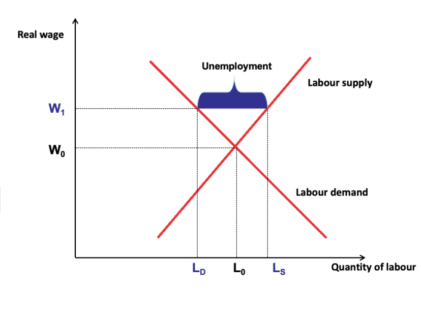
Sticky wages an involuntary unemployment

• Start at equilibrium: real wage W0, employment L0
• Deflation with sticky wages raises the real wage to W1 > W0
• At W1, firms demand only LD while workers supply LS
• The gap LS – LD is involuntary unemployment: people willing to
work at the going wage cannot find a job
• It persists as long as the real wage cannot fall back to W0.
• Keynes's remedy: raise aggregate demand and prices

productivity kept growing

• While unemployment rose, output per hour of those who kept their jobs continued to increase
• Western Europe: 1.56% a year in 1913–50, the same pace as 1870–1913 (1.55)
• US: faster than before 1914 (2.48 vs 1.92), so its lead widened
• Japan: slowed (1.80 vs 1.99)
• All far below the golden age (Western Europe 4.77; Japan 7.74)

Why did productivity keep growing, and why does it
matter?
Three plausible explanations
• Technology: many 'second industrial revolution' inventions (internal
combustion engine, Ford's assembly line, electrical network and
motor) had a measurable aggregate effect only during or after the war
• Human capital: continued expansion of primary and secondary
education and investment in higher education, with a lagged effect on
productivity
• Composition (1930s): layoffs hit the least productive workers first,
which raised measured average productivity
Why it matters
• Slow growth and depression were man-made (e.g. war), not ‘natural'
• Helps explain the post-1945 boom: once man-made obstacles were
removed, Europe could exploit a large backlog of technology and
human capital

The role of technology

• Recall biased technical change
• Growth after 1900 was driven by new industrial technologies
• New technologies were more capital- and knowledge-intensive
→ biased technical change
• Industrialised countries rich in capital and human capital grew faster
• General purpose technologies
• Electrification: power supply; electric motors, railways, trams; lighting
(round-the-clock production)
• Motorisation: faster ships and diesel locomotives; new modes of
transport (road and air)
• The US led in both

Summary

• World War I was a watershed: the end of the 'long' 19th century and of the first globalisation, followed by a global pandemic
• 1913–1950 was a pause in modern economic growth: a slowdown
everywhere except the USSR, sharpest in Western Europe; a decent
1920s, a dismal 1930s
• Globalisation backlash: technology favoured integration, politics
reversed it (trade, migration, capital)
• Mass, persistent unemployment: voluntary (classical; Benjamin and
Kochin) or involuntary (Keynes: sticky wages, overvalued sterling,
demand shocks)?
• Technological progress and productivity growth continued, so the
slowdown was man-made; it left a backlog for the post-1945 boom
• Key concepts: modern economic growth, globalisation backlash,
voluntary vs involuntary unemployment, 'sticky' wages, general purpose technology, biased technical change