2. Feedforward Neural Networks

What is Feedforward Neural Network (FNN) and what its main goal?

• FNN: maps inputs directly to outputs through a sequence of computational layers

  • information flows forward from input to output

  • Hidden layers learn intermediate representations

  • 2 important goals are expressiveness (what func the network can be represent) and trainability(how reliably it can learn them)

What is linear model and what its main limitation?

Linear model computes:

*form in pict

• x = input

• W = weights

• b = bias

• y(hat) = prediction

→ Linear model are simple and efficient but they cannot represent arbitrary nonlinear relationships

What is linear decision boundary?

For binary classification, the equation:

*form in pict

→ defines a linear decision boundary

• it separates classes using a straight line(in 2D) or a hyperplane(in higher dimensions)

• Some datasets are linearly seperable, while other require more complex decisions regions

What is XOR problem, and why can’t a single linear model solve it?

XOR output:

• 1 when 2 binary inputs are different

• 0 when they are the same

→ a single straight line cannot seperate 2 output classes

→ so, XOR demonstrates why neural networks need nonlinear computation

What is perceptron and how does it make predictions?

Perceptron: a trainable linear decision unit

• it computes: *form in pict

  followed by decision function

  • each inputs contribute through a learned weight

  • Weighted inputs are combined

  • The bias shifts the decision boundary

  • Training changes w and b

How do weights and bias affect the decision boundary ?

• weights, w, determine the boundary’s orientation

• Bias, b, determine its position

• Changing these parameters changes model’s decision rule

  → learning means changing these decision boundary

Why is stacking multiple linear layers without activation functions insufficient?

*form in pict

• Therefore, multiple linear or affine layers without nonlinear activations are equivalent to 1 affine transformation

• Depth alone is not enough!!

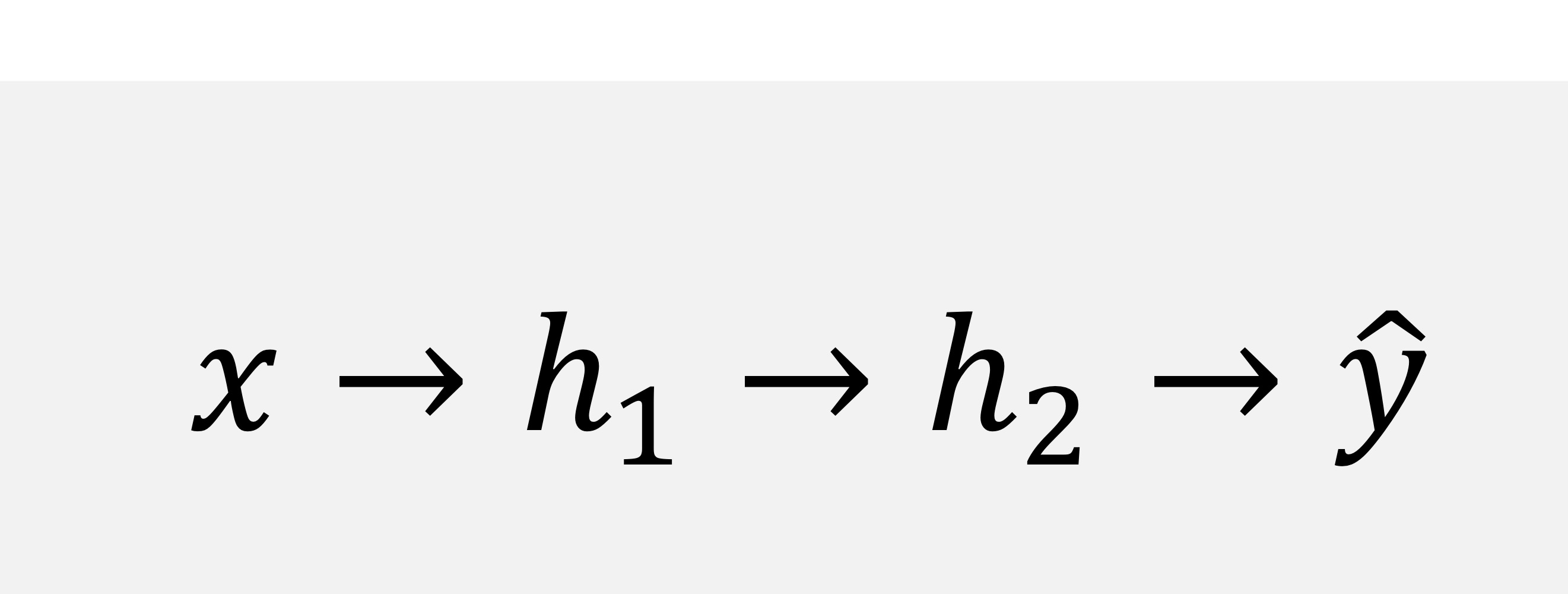
What are hidden layers, and why are they useful?

Hidden layers: lie between input and output layers

• Through transform representation step by step:

  x → h1 → h2 → y(hat)

• Instead of predicting directly from input, the network learns intermediate features that help solve complex problems

What is Multi-Layer Perceptron(MLP) and what are its 2 essential components?

MLP: combines linear transformations and nonlinear activation functions

For one hidden layer:

*form in pict

Its 2 essential components are:

1. Linear Transformations → combine and transform features

2. Nonlinear activations → allow complex nonlinear relationships

=> together, they create a more expressive function

Why do neural networks need nonlinear activation functions?

• without nonlinear activation functions:

  Linear → Linear → Linear = Still linear

• With nonlinear activations:

  Linear → Nonlinear → Linear = Can represent nonlinear functions

  => activation functions make depth meaningful by allowing network to learn complex patterns and decision boundaries

What is the Sigmoid activation function, and its properties?

*form in pict

• Output range: (0,1)

• Useful for interpreting outputs as probabilities

• Saturates for very large positive or negative inputs

• Saturation can cause small gradients, making learning difficult

What is the Tanh activation function, and its properties?

*form in pict

• Output range: (-1,1)

• Produces zero-centerd outputs

• Like Sigmoid, it can suffer trom saturation

=> Main difference: Tanh is zero-centered, while Sigmoid outputs only positive values

What is ReLU and why is it widely used?

*form in pict

• Negative inputs bcm 0

• Positive inputs remain unchanged

• Computation is simple and efficient

• Positive activations avoid the same saturation behavior as Sigmoid and Tanh

→ ReLU is a standard activation in many DL networks

What is theDying ReLU problem?

Dying ReLU occurs when a neuron remains in the negative-input region

• Because ReLU outputs 0 for negative input, its gradient is also 0

• As a result, the neuron may stop receiving gradients and fail to learn

What is Leaky ReLU and how does it differ from Dying ReLU?

*form in pict

• Unlike standard ReLU, Leaky ReLU allows small nonzero gradient for negative inputs

• This helps reduce the Dying ReLU problem while preserving a simple piecewise-linear structure

What is network depth, and what happens when depth increases?

Depth: number of sequential computational layers or stages

x → h1 → h2 → … → hL → y(hat)

Increasing depth provides:

• More stages of transformation

• More opportunities for intermediate representation

• More complex function composition

What is network width, and what happens when width increases?

Width: Number of hidden units or features within a layer

* From the picture

→ hidden representation has 512 features

• Increasing width provides more parallel representational capacity within the same computational stage

What is the difference between network depth and width?

• Depth = more transformations

• Width = More features

What are hierarchical representations in deep learning?

Deep networks can gradually build complex features from simpler ones

• For image recognition:

  Pixels → Edges → Shapes → Objects

  • Early layers learn simple features

  • Intermediate layers combined them

  • Later layers form task-relevant representations

• Later layes operate on features learned by earlier layers

Why can deep neural networks be viewed as compositions of functions?

• Each layer performs a transformation, and its output becomes the input to the next layer

  *form in the picture

• This allows complex functions to be constructed from simpler functions

• Depth changes the structure of computation, not just the number of parameters

What is Universal Approximation and what does it NOT guarantee?

Universal Approximation states that sufficiently large nonlinear neural network can approximate a broad class of functions

• it demonstrates the network’s expressive power

• However, it does NOT guarantee:

  • how large the network must be

  • Easy optimisation

  • Sufficient training data

  • Good generalisation to unseen data

=> Expressive ≠ Easy to Train

Why do the output layer and loss function depend on the prediction task?

Different task required different types of predictions and error measurements

• 3 Common tasks:

  • Regression → Continuous value

  • Binary classification → Two classes

  • Multiclass classification → Multiple classes

• For each task, we decide what the model outputs, how to interpret it, and how to measure its error

=> Task → Output → Loss

What is regression and what output does it require?

Regression: Predicts continuous numerical values

e.g:

• House prices

• Temperatures

• Demand forecast

*typical output in pict

=> The final layer directly produces a continuous value, so no probability transformation is required

What is Mean Squared Error (MSE) and why is it used for regression?

MSE: measures the average squared deifference between predictions and targets

*form in pict

• Correct prediction→ 0 error

• Large errors receive large penalties

• Commonly used for continuous regression

=> Regression → Continuous Output → MSE

What is binary classification and how does Sigmoid help?

Binary classification: predicts btw 2 classes, such as spam/not spam or disease/no disease

• the model produces one raw score called a logit, *in pict

• Sigmoid converts it into a probability:

  *in pict

• The resulting probability lies between 0 and 1

What is Binary Cross-Entropy(BCE) and how does it penalize predictions?

BCE: Measures prediction error for binary classification

*form in pict

• correct, high-confidence prediction → low loss

• Incorrect, high-confidence prediction → high loss

=> it encourages predicted probabilities to move toward the correct labels

What is ‘nn.BCEWithLogitsLoss()’ and why is it preferred in PyTorch?

‘nn.BCEWithLogitsLoss()’ combines:

Sigmoid + Binary Cross-Entropy

• it:

  • accepts raw logits

  • Internally performs the necessary calculations

  • Provides better numerical stability

• Therefore, you should not manually apply Sigmoid before passing logits to this loss function

What is multiclass classification and how does Softmax work?

Multiclass classification predicts among K classes

• The model produce K logits, one for each class

• e.g: z = [2.1,-0.4,0.8]

  Softmax converts them into class probabilities:

  *form in pict

• The probabilities sum to 1, and higher logits correspond to higher probabilities

How do regression, binary classification, and multiclass classification differ in output and loss?

• Regression use prediction directly

• Binary classification interprets logit through Sigmoid

• Multiclass classification use Softmax probabilities

Why is weight initialisation important before training begins?

Every weight needs an initial value before training

Initialisation affects:

• Activation magnitude

• Gradient magnitude

• Whether neuron can learn different features

• Stability of signals across layers

Poor initialisation can make training difficult even with a good architecture

Why shouldn’t all hidden-layer weights be initialised to 0?

Initialising all hidden neurons identically creates a symmetry problem

Identical neurons:

1. Receive identical inputs

2. Produce identical outputs

3. Receive identical gradients

4. Remain identical after updates

→ Therefore, random initialisation breaks symmetry, allowing different neurons to learn different features

What happens when initial weights are too small or too large?

Weight too small:

• Activation may shrinks across layers

• Information can gradually disappear

Weight too large:

• Activation may grow rapidly

• Computation may become unstable

→ Good initialisation maintains a useful signal scale throughout the network

What is the difference between Xavier and He initialization?

Xavier/Glorot initialization:

• Designed to preserve signal scale

• Commonly associated with Sigmoid and Tanh networks

He/Kaiming initialization:

• Account for the behaviour of ReLU-like activations

• Commonly used in ReLU-based networks

→ initialisation should reflect both layer size and activation function

Why can gradients become unstable when travelling through deep networks?

• Backpropagation repeatedly applies the chain rule

• The gradient for an early parameter depends on products of many local derivatives

• If this derivatives repeatedly have magnitude that are too small or too large, the gradients may vanish or explode

• This affects whether useful learning signals reach earlier layers

What are vanishing gradient and why do they make learning difficult?

Vanishing gradients: occur when gradients become extremely small during backpropagation

• For example: 0.5×0.5×0.5×… → 0

• Consequences:

  • Earlier layers received tiny ingredients

  • Parameter updates become very small

  • Learning in early layers becomes ineffective

What are exploding gradient and how do they affect training?

Exploding gradient: occur when gradient become extremely large

• For example: 2×2×2×… → Very large

• Consequences:

  • Parameter updates become unstable

  • Loss may oscillate

  • Training may diverge

What is the difference between underfitting and overfitting?

Underfitting:

• Training performance is poor

• Validation performance is also poor

• The model has not learned the underlying relationship adequately

Overfitting:

• Training performance is very good

• Validation performance is much worse

• The model learn training-specific patterns that do not generalise well

How does model capacity affect generalisation?

Increasing model capacity generally allows the model to fit training data better

However:

• Training error often decreases

• Validation error may decrease initially then increase

• Excessive capacity can make overfitting easier

The goal is not simply no training error but good performance on unseen data

What is regularisation and why is it needed?

Regularisation: Modify training to discourage and desirable solutions

The goals are to:

• Reduce overfitting

• Improve generalisation

• Encourage robust representations

  
  

Common methods include:

• Weight decay

• Dropout

• Early stopping

What is weight decay and how does it help regularisation?

Weight decay: Discourage excessively large parameter values

• L2-regularization intuition:

  *form in pict

• This encourages less extreme perimeter configurations

• Some modern optimisers implement weight decay differently from a direct L2 penalty

What is dropout and how does it differ between training and inference?

Dropout: randomly sets some hidden activations to zero during training.

• This prevents the model from depending on the same neurons every time.

• Training: Random subsets of neurons are disabled, effectively training different subnetworks.

• Inference: The full network is used.

→ Dropout helps reduce overfitting.

What is early stopping, and why is it useful?

Early stopping: monitors validation performance during training.

• Training loss may continue decreasing even after validation loss stops improving.

• Continuing too long may cause overfitting.

• Early stopping prevents training far beyond the point where validation performance is useful.

What should we examine when analyzing training and validation curves?

Examine:

1. Training loss → how well the model fits training data

2. Validation loss → how well it performs on held-out data

3. Gap between curves → possible generalization problems

4. Trends → whether either curve is improving or becoming unstable

=> these patterns help diagnose training problems

How can training curves reveal healthy training, underfitting, overfitting, or optimization failure?

These are useful diagnostic patterns, not absolute rules.

What actions can improve different training problems?

• Healthy training: Continue or monitor

• Underfitting: Consider more model capacity or better optimisation

• Overfitting: Use regularisation or early stopping

• Optimisation failure: Check learning rate, initialisation, and gradients

=> Training curve help distinguish architecture, optimisation, and generalisation problems

How is an MLP implemented in PyTorch, and what does each layer do?

• fc1 transforms 784 → 256 features.

• fc2 transforms 256 → 128 features.

• fc3 transforms 128 → 10 output logits.

• F.relu() adds nonlinearity after the first two layers.

How do tensor shapes changes through this MLP?

For batch size B:

[B,784] → [B,256] → [B,128] → [B,10]

• Linear layers change the feature dimension

• ReLU preserves the tensor shape

• The final dimension corresponds to the 10 classes

=> an important skill is predicting the tensor shape after every layer

Why is Softmax not required before ‘nn.CrossEntropyLoss()’?

• The model returns 10 raw logits per example.

• ‘CrossEntropyLoss’ internally performs the necessary normalization and loss calculation.

• Therefore, adding Softmax before it is unnecessary.

• The loss transforms the logits of shape [B, 10] into a scalar loss by default.

=> [B,10] → CrossEntropyLoss → Scalar Loss

How does the MLP connect to the PyTorch training loop?

• The training principle remains the same as Lecture 1:

Clear gradients → Forward pass → Loss → Backward pass → Update

• The difference is that model(x) now represents a multi-layer nonlinear function, and backpropagation automatically computes gradients through its differentiable layers.

What makes a Multi-Layer Perceptron powerful, trainable, and able to generalize?

A useful MLP needs three qualities:

1. Expressiveness

Depth + Width + Nonlinearity

These provide nonlinear decision boundaries, intermediate representations, hierarchical computation, and high functional capacity.

2. Trainability

Initialization + Stable Gradients + Optimization

These help the network learn reliably.

3. Generalization

Appropriate Capacity + Regularization + Validation

These help the model perform well on unseen data.

Core idea: A successful neural network must be expressive enough to represent useful functions, trainable enough to learn them, and regularized enough to generalize.