5- Community ecology

Vocabulary practice cards focusing on herbivore interactions, plant chemical and structural defenses, primary and secondary ecological succession, and food web complexity metrics.

Primary succession

The sequential change and establishment of plant and animal communities on newly exposed substrates that completely lack living organisms and organic soil, such as bare rock, volcanic lava, sand dunes, or glacial meltwater ponds.

which is the ecological process of life establishing itself in an environment for the very first time.

• Left Image (Nunataks/Glacial Retreat): This shows bare mountain peaks sticking out through a massive ice sheet. As glaciers melt and retreat, they uncover raw, scoured bedrock that has been buried for thousands of years. This bare rock contains no organic matter, making it a perfect textbook setting for primary succession to begin.

• Right Image (The Cordilleran Ice Sheet Map): This satellite map illustrates western North America (including Alaska, Yukon, Haida Gwaii, and Vancouver Island) during the Glacial Maxima 15,000 years ago compared to recent times. As this massive ice sheet retreated northward, it left behind vast expanses of bare rock, sediment, and glacial lakes—triggering widespread primary succession across the Pacific Northwest.

whats happening in this picture:

This slide uses the famous 1980 eruption of Mount St. Helens to illustrate how a major ecological disaster completely resets a landscape, creating a textbook environment for primary succession.

whats happening in this picture:

This slide demonstrates primary succession occurring on bare rock exposed by landslides on the rugged west coast of Vancouver Island.

This slide demonstrates primary succession occurring on bare rock exposed by landslides on the rugged west coast of Vancouver Island.

• Nitrogen Fixation: Bare rock slides contain virtually zero soil nutrients. Alders possess specialized root nodules containing symbiotic bacteria that pull nitrogen directly from the air, allowing them to grow where other plants would starve.

• Soil Building: As the alders grow, they shed nutrient-rich leaves every autumn. This decomposing organic matter gradually accumulates on top of the rocks, building the very first layers of new, fertile soil.

• Paving the Way: Over decades, the soil built by the alders becomes deep and rich enough to support the seeds of larger, long-lived conifers (like Western Redcedar and Sitka Spruce), slowly returning the slope to a mature forest.

whats ecological succession:

the sequential change in species composition of the community over time

Secondary succession?

explain the image

whats seral stage?

wats duration?

change of an established community

The sequential progression and directional change of an established biological community following a disturbance, such as a shallowing pond accumulating sediment, pollen, and leaves until it transitions into terrestrial forest.

the image explains:

process of aquatic-to-terrestrial succession (often studied as a hydrosere), tracking how an established body of water transitions into dry land over time.

The central illustration demonstrates the sequential timeline of a lake filling in:

• Top Stage (Open Water Lake): A newly formed basin (often originating from melting glacial ice over glacial till/soil) fills with water. It starts deep, with clear open water and a clean basin.

• Middle Stage (Sediment Accumulation): Over centuries, the lake gradually collects organic and inorganic materials like sediment, pollen, and leaves. As the water gets shallower:

  • Shoreline plants like reeds, grasses, and herbs move inward.

  • Submerged and floating aquatic plants multiply, speeding up the accumulation of dead plant matter on the bottom.

• Bottom Stage (Terrestrial Transition): Larger woody plants and shrubs gradually colonize the marshy borders, displacing the grasses. Eventually, trees take root, fully converting the ancient lake basin into a stable terrestrial forest community.

---

Seral Stage: Each temporary, sequential community that replaces the one before it is called a seral stage (e.g., the open water stage, the reed/marsh stage, and the shrub stage are all individual seral stages).

• Duration: The slide notes that successive seral stages last longer than the stages that came before them, with the final terrestrial forest being the most stable and long-lasting community.

---

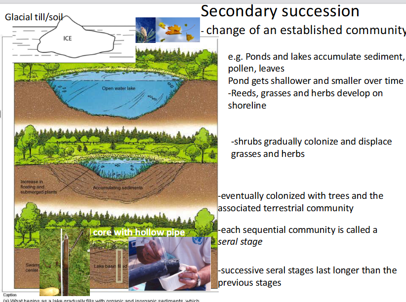
Seral stage

A discrete, sequential transitional community occurring during ecological succession, where successive stages typically persist for longer durations than earlier ones.

Each temporary, sequential community that replaces the one before it is called a seral stage

explain this

This slide explains palynology (the study of fossil pollen) and ancient DNA tracking, which are the primary scientific methods used to reconstruct historical plant communities and climates over thousands of years.

---

The chart shows a real pollen core record from Langford Lake (located right near Victoria, BC) spanning back roughly 10,000 years Before Present (BP):

• The Y-Axis (Depth/Time): The top represents the modern day (\(0.0\) meters), while the bottom (\(7.0\) meters deep) goes back \(10,000\) years. As you go deeper down the core, you travel further back in time.

• The X-Axis (Pollen Percentages): The width of each tree's curve shows how abundant its pollen was at that time.

• Shifts in Forest Composition: At the very bottom (\(10,000\) years ago), the landscape was dominated by Lodgepole pine (Pinus contorta), signaling a cooler, post-glacial climate. Over time, the climate warmed, and species like Douglas fir and Western hemlock expanded, while pine declined.

• Volcanic Ash Marker: The distinct horizontal line around \(3.2\) meters represents a historic volcanic ash layer (likely from Mount Mazama/Crater Lake eruption about \(7,600\) years ago), which serves as a perfect time-stamp across regional sediment cores.

---

2. The Methodology: Radiocarbon Dating (\(^{14}\text{C}\))

To know exactly when these plant shifts happened, scientists date the organic material in the core layers:

• Carbon has three main isotopes: \(^{12}\text{C}\) (\(98.9\%\)), \(^{13}\text{C}\) (\(1.11\%\)), and the unstable, radioactive \(^{14}\text{C}\) (only 1 atom per trillion).

• When a plant dies, it stops absorbing carbon. The unstable \(^{14}\text{C}\) steadily decays into \(^{14}\text{N}\) with a known half-life of 5,730 years.

• By measuring how much \(^{14}\text{C}\) is left in a specific layer of the core, scientists can calculate the exact historical age of when those plants died.

---

3. Modern Tech: eDNA & sedaDNA

While pollen tracking is highly effective, the slide notes that cutting-edge molecular tools are expanding what we can learn from these mud cores:

• eDNA (Environmental DNA): Cellular debris left behind in the environment (soil, water) by living organisms.

• sedaDNA (Sedimentary Ancient DNA): Ancient DNA preserved inside the deep sediment layers.

• The Benefit: By amplifying tiny fractions of this ancient DNA, scientists no longer rely solely on visible pollen grains. They can precisely identify both animal and plant species that inhabited the area thousands of years ago.

explain this

what r the 4 stages about

wha happens with disturbances?

what r the 2 types of succession drivers?

what happens if disturbances continues?

what happens if they dont continue?

This slide provides a comprehensive model of ecological succession, showing how ecosystems progress linearly through development stages while highlighting that disturbances can reset or loop an ecosystem back to earlier stages at any time.

1. The Core Progression of Succession

The straight horizontal path along the middle of the diagram illustrates the theoretical sequence of an ecosystem building complexity:

• Bare Ground: The ultimate starting point. This is triggered by extreme events like retreating glaciers or volcanic eruptions (Primary Succession).

• Pioneer Seral Stage: The first hearty organisms (like lichens, mosses, or specialized grasses) move in to colonize the barren landscape and start building soil.

• Seral Stages: The intermediate communities that progressively displace the pioneers. Shrubs and fast-growing trees populate the area (Secondary Succession).

• Climax: The final, stable, and self-sustaining community (typically a mature forest) that remains balanced until a major event disrupts it.

2. The Impact of Disturbances (The Lower Return Curved Arrows)

The key takeaway of the slide is written directly at the bottom: "Disturbance can reset any seral stage back to any other stage." The multi-colored curved arrows moving from right to left show that succession is rarely a perfect one-way street:

• A severe wildfire, landslide, or human logging can strike a late Seral Stage or Climax forest and completely strip it down to Bare Ground, resetting it all the way back to the beginning.

• Alternatively, a minor disturbance might only knock a Climax community back a few steps into an intermediate Seral Stage or Pioneer Stage rather than destroying it entirely.

---

3. Types of Succession Drivers

The slide breaks down succession pathways into two core mechanisms based on what causes the change:

• Allogenic Succession (Driven by Abiotic Disturbance): Environmental changes caused by non-living forces. The photo of the devastating forest fire represents an abiotic force that acts externally to reset the ecosystem.

• Autogenic Succession (Driven by Biotic Disturbance/Processes): Environmental changes driven directly by the living organisms within the community. The photo of the beaver building a dam represents a biotic disturbance; the animal's physical actions flood the forest, altering the local environment and intentionally forcing a shift in the local plant and animal seral stages.

4. Cyclic Succession Loops (The Circular Arrows)

• Possible cyclic succession if disturbances continue: If an ecosystem experiences recurring, regular disturbances (like frequent small fires or seasonal flooding), it gets locked in a loop within the intermediate Seral Stages, never allowed to grow into a climax community.

• Possible cyclic succession if no disturbances: Even in a stable environment without external disasters, dominant species within a Climax community eventually grow old, die, crash, and regenerate, creating localized internal birth-and-death cycles.

---

Allogenic succession

A succession process driven primarily by external, abiotic environmental disturbances or geophysical factors, such as landslides, volcanic eruptions, or windstorms.

Autogenic succession

A succession process driven internally by biotic changes that organisms themselves bring about within their habitat, such as dam-building activity altering hydrology and plant communities.

explain this

This slide displays a graph illustrating the typical relationship between species richness and the progression of successional time (seral stages) in most ecological communities.

---

• Y-Axis (# species): Represents species richness, which is the total number of different species living in the ecosystem.

• X-Axis (Time- seral stage): Tracks the passage of ecological time as the ecosystem transitions from early pioneer stages toward a mature climax stage.

The green line breaks down the ecological trend into two distinct phases:

• Phase 1: The Linear Increase (Early to Mid-Succession): As time passes, the line climbs steadily upward. This shows that species richness increases during the early and intermediate seral stages. As pioneer species build soil and alter the microclimate, they create new ecological niches. This allows a diverse wave of new plants, insects, and animals to move in and colonize the area alongside the existing species.

• Phase 2: The Plateau (Late Succession / Climax): Eventually, the green line flattens out. When the ecosystem reaches its mature, late seral stages (approaching the climax community), the total number of species stabilizes and levels off. At this stage, the available niches are largely filled, and dominant, long-lived species (like canopy trees) establish structural stability, preventing rapid new arrivals.

---

he slide explicitly labels this pattern as applying to "most communities." While this linear rise and plateau serves as the baseline model, other ecological models (like the Intermediate Disturbance Hypothesis) suggest that species richness can sometimes peak in the middle stages and slightly drop during the final climax stage due to intense competition from dominant species.

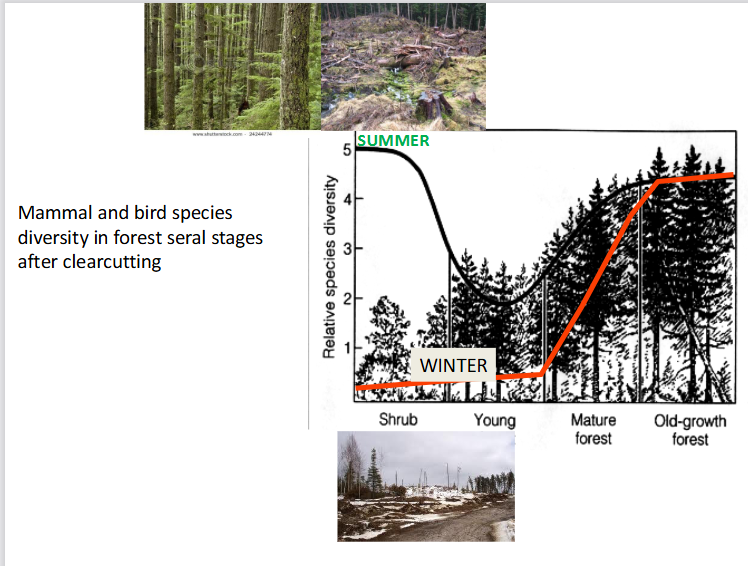
explain

This slide illustrates how mammal and bird species diversity changes across different forest recovery stages (seral stages) following a clearcut, highlighting a dramatic difference between summer and winter habitat value

While early successional stages (Shrub) provide an excellent temporary food source during the summer, mature and old-growth forests are structurally irreplaceable for maintaining high wildlife diversity year-round, especially for winter survival.

2. The Summer Trend (Black Line)

In the summer, wildlife diversity follows a U-shaped curve:

• High in Shrub Stage (Rating ~5): Right after clearcutting, sunlight floods the ground. This triggers a massive flush of berries, seeds, shrubs, and insects, attracting a wide variety of nesting birds and foraging mammals.

• Drop in Young Forest (Rating ~2): As young trees grow closely together, their canopy closes completely. This blocks out the sun, killing off the forest-floor shrubs and plants. Food disappears, creating a "green desert" where summer diversity bottoms out.

• Recovery in Mature & Old-Growth: As the forest ages and trees naturally die or fall, gaps open in the canopy. Structural complexity returns, causing summer diversity to rise back up.

---

3. The Winter Trend (Red Line)

In the winter, wildlife diversity follows a completely different, delayed upward curve:

• Very Low in Shrub & Young Stages (Rating <1): Even though the shrub stage is great in the summer, it has zero canopy cover. In the winter, it gets buried in deep snow and exposed to freezing winds, making it unusable for most wildlife.

• Steep Rise in Mature Forest: Diversity climbs rapidly as trees grow large enough to provide shelter.

• Peak in Old-Growth Forest (Rating ~4.5): Old-growth forests are absolutely vital for winter survival. Their massive, multi-layered tree canopies catch falling snow before it hits the ground, leaving the forest floor clearer for animals to move around and find food. They also provide essential thermal cover (protection from the freezing wind and cold).

---

explain the 4 stages

whast the law of constant yield?

This slide illustrates the Bormann-Likens Biomass Accumulation Model, which tracks how total forest biomass (both living and dead organic matter) changes over time following a severe disturbance like clearcutting. [1]

1. Understanding the Four Phases of Biomass Succession

The model breaks forest development down into four distinct phases:

• 1. Reorganization: Immediately after a clearcut, total ecosystem biomass actually drops slightly. Even though new weeds and shrubs begin growing, the rapid decomposition of the leftover dead branches, roots, and logging slash outweighs any new living plant growth.

• 2. Aggradation: This is the longest phase, marked by a steep, rapid accumulation of biomass. The young, fast-growing tree canopy closes and gathers maximum structural mass. It reaches a peak when the initial even-aged cohort of trees hits maturity.

• 3. Transition: Total biomass declines from its peak. During this phase, the large trees from the original post-clearcut generation begin to grow old and die off. This initial heavy wave of mortality causes a temporary drop in overall standing wood mass, which isn't immediately replaced by the smaller, younger understory trees.

• 4. Steady State: Biomass levels out and oscillates around a stable baseline. The forest becomes a uneven-aged, shifting mosaic. As individual old trees die and fall, new gaps open for localized growth, creating a perfectly balanced structural equilibrium across the landscape over centuries.

In ecology, this law states that once a plant community reaches high enough densities, the total biomass yield reaches a plateau and remains constant, regardless of further increases in initial planting density

explain this

This slide demonstrates how the length of time required to reach late seral (climax) stages varies dramatically by region, proving the ecological rule that the rate of succession is positively correlated to temperature and rainfall.

• Warm and Wet = Fast Succession: Ecosystems with high temperatures and heavy rainfall have rapid metabolic, decomposition, and plant growth rates. Soil forms quickly, and biological communities change rapidly.

• Cold and Dry = Slow Succession: Ecosystems with freezing temperatures and low precipitation develop at a snail's pace because plant growth is limited and soil development takes thousands of years.

Case study 1: Krakatau, Indonesia (-100 years)

• The Disturbance: In 1883, the volcanic island of Krakatau exploded violently, burying the entire island under 15 meters of sterile, blistering hot lava rock. It was a complete reset down to bare ground (primary succession).

• The Recovery: Because Indonesia is a tropical environment with intense heat and massive rainfall year-round, life recovered at an astronomical speed. Within just ~100 years (as shown in the lower-left photo), the bare volcanic rock completely transformed back into a lush, dense tropical rainforest.

Case study 2: Coastal BC rainforest (100-1000 years)

• The Timeline: In the temperate, wet climate of the Coastal British Columbia rainforest, individual trees take roughly 100 years to grow large following a disturbance. However, establishing a true, structurally complex old-growth forest takes up to 1,000 years.

• Indicator Species: The slide references the Marbled Murrelet, a rare seabird that strictly relies on these ancient, 1,000-year-old canopy structures. They require the massive, wide, moss-covered branches of old-growth trees to lay their eggs, meaning they cannot survive in a simple 100-year-old second-growth forest.

Case study 3: the Yukon (10000 years)

• The Timeline: The subarctic environment of the Yukon is incredibly cold and receives very little annual precipitation.

• The Recovery: As shown by the map of the Cordilleran Ice Sheet melting 15,000 years ago, it takes roughly ~10,000 years for this harsh, frozen climate to progress through succession stages to achieve a stable landscape. The lack of heat and water severely bottlenecks soil building and plant development, making ecosystem recovery an incredibly slow process.

Facilitation

A successional mechanism where early colonizing species alter environmental conditions to make the site more suitable for subsequent species but less favorable for themselves, such as nitrogen-fixing clover enriching soil before being shaded out by trees.

. The Visual Example: Clover vs. Trees

The bottom half of the slide maps out a perfect real-world example of facilitation in action:

• Step 1: The Clover Moves In: Following a disturbance, Clover (a pioneer plant) rapidly carpet-bombs the open ground (bottom-left photo).

• Step 2: Soil Improvement: Clover is a nitrogen fixer. It pulls nitrogen gas out of the air and converts it into a usable soil nutrient. As the clover grows, dies, and decomposes, it steadily adds Nitrogen (N) and organic matter to the raw, nutrient-poor soil.

• Step 3: The Climax Takeover: The now rich, nitrogen-heavy soil provides the exact fertile environment required for tree seeds to take root and grow into a young forest (bottom-right photo).

• The Twist (Self-Elimination): As the trees grow tall and form a dense canopy, they block out the sun. Because clover requires direct sunlight to survive, the trees completely shade out the clover. The clover facilitated the trees' growth, but in doing so, engineered its own local extinction (represented by the green clip art and scissors icon).

what r stochastic events:

• Definition: These are random, largely unpredictable events—such as wind currents blowing a specific seed cloud into an open patch of dirt (illustrated by the top-right photo of blowing tree seeds/pollen).

• The "First Come, First Served" Rule: Whichever species happens to land in the empty space first gets a massive head start. They grab the available sunlight, water, and nutrients, successfully establishing themselves simply due to lucky timing.

• When It Matters Most: This mechanism is most important in early seral stages, right after a disturbance has cleared a landscape and left open, empty niches.

---

Inhibition

A successional mechanism where early established species actively hinder, delay, or prevent colonization by subsequent species through competitive exclusion or the release of allelopathic chemicals, prolonging the current seral stage.

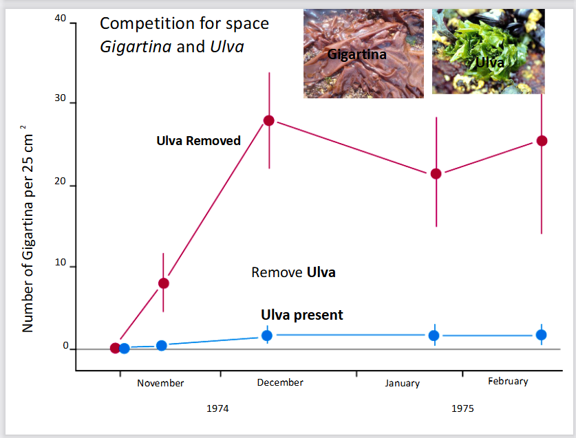
explain this graph

This slide illustrates the successional mechanism of inhibition using a classic marine ecology experiment that tracks competition for intertidal rock space between two species of algae: Ulva (sea lettuce) and Gigartina (red algae).

1. The Core Concept: Inhibition

Unlike facilitation (where an early species modifies the environment to help a later species), inhibition occurs when early colonizers monopolize resources and actively prevent other species from establishing. Succession can only progress further when a disturbance or natural mortality damages or removes these early dominant species, freeing up resources.

---

2. Breakdown of the Experiment Graph

The graph tracks the number of Gigartina individuals per 25 cm² from November 1974 to February 1975 under two experimental conditions:

• Blue Line (Ulva present): In control plots where Ulva is allowed to grow naturally, the number of Gigartina remains flatlined near zero. Ulva is a rapid early colonizer that completely blankets the rock surface, physically blocking Gigartina spores from settling and growing.

• Red Line (Ulva removed): In experimental plots where scientists manually removed Ulva, the Gigartina population instantly exploded. It jumped from zero in November to nearly 30 individuals by December.

---

3. Ecological Conclusion

The experiment proves that Gigartina does not require Ulva to prepare or "facilitate" the substrate to survive. Gigartina is fully capable of thriving on its own from the beginning, but its appearance in natural succession is normally bottlenecked and inhibited by Ulva's aggressive competition for physical space.

Connectance ($C$)

An index of food web complexity calculated as the actual number of trophic links ($L$) divided by the total number of theoretical possible links ($N$), expressed as $C = \frac{L}{N}$.

whats tolerance??

• Under this model, species replace one another over time because later-stage species are better adapted to tolerate the changing environmental pressures (such as increased shade, crowding, or reduced ground-level food) than early-stage species.

just list the 4 ecological mechanisms for succession

• stochastic events

• facilitation

• inhibition

• tolerance

Number of possible links ($N$)

The maximum theoretical number of binary trophic links in a food web consisting of $n$ distinct species, calculated using the formula $N = \frac{n(n - 1)}{2}$.

sedaDNA (sedimentary ancient DNA)

Genetic material isolated and amplified from perennially frozen and dated sediment cores, used to detect the presence of historical taxa and reconstruct regional biodiversity.

Ghost ranges

Temporal intervals during which dwindling populations persisted in localized refugia despite being completely undetected in the macrofossil bone and tooth record.

Nepetalactone

A growth hormone mimic and secondary metabolite produced by catnip (mint family) that deters cockroaches and beetles, disrupts insect moulting, and attracts aphid-consuming lacewings.

Urushiol

An oily organic contact allergen secreted by poison ivy as a chemical defense mechanism, triggering acute skin irritation and contact dermatitis in sensitive animals.

Proteinase inhibitors

Defensive biochemical compounds found in plants such as cotton, chickpea, and potato that disrupt herbivore digestion by interfering with the breakdown of dietary proteins.

Mixed function oxidase

An animal metabolic enzymatic system that breaks down and neutralizes toxic plant secondary compounds through oxidation, reduction, and hydrolysis.

Radiocarbon dating

A radiometric technique that estimates the age of organic material by measuring the remaining quantity of radioactive $^{14}\text{C}$, which has a half-life of $5730\text{ years}$ and decays into $^{14}\text{N}$.

Assembly rules

Deterministic ecological constraints specifying the sequential order in which species can colonize a habitat; for example, predators cannot establish until prey are present.

Allelopathy

A form of chemical inhibition where a plant produces and releases bioactive secondary compounds into the soil to inhibit the growth, germination, or survival of neighboring plant species.

Primary producer, 1 consumer, 2 consumer, 3 consumer

what r the trophic levels

Primary producer: An autotrophic organism situated at the base of an ecological food pyramid or chain, such as terrestrial trees or marine phytoplankton, that manufactures biomass directly from inorganic nutrients and sunlight.

1 consumer: An herbivorous organism that occupies the second trophic level by directly consuming primary producers, such as a caterpillar eating leaves or krill grazing on phytoplankton.

2 consumer: A carnivorous or predatory organism that feeds on primary consumers within a food web, such as a warbler that preys upon caterpillars.

3 consumer: A top predator situated on the fourth trophic level that preys upon secondary consumers, such as a hawk consuming insectivorous birds or an orca consuming marine mammals.

Devil's club

A temperate underbrush plant characterized by dense mechanical spines and prickles covering its stems, serving as physical structural defenses against browsing herbivores.

Himalayan blackberry

A vigorous bramble that utilizes sharp epidermal prickles along its canes as structural defenses to protect its foliage and berries from large herbivores.

Peyote (Lophophora williamsii)

A small spineless cactus that synthesizes mescaline, a psychoactive alkaloid secondary metabolite that deters browsing herbivores by modifying nervous system function.

Poison dart frog

A brightly colored amphibian capable of bioaccumulating and concentrating toxic chemical alkaloids derived from its dietary prey as a lethal chemical defense against predation.

Green lacewing

A predatory insect that is attracted to volatile plant compounds such as nepetalactone and feeds on aphids, providing indirect protection to plants.

Beaver

A semi-aquatic rodent that functions as an agent of autogenic succession by felling trees and building dams, creating ponds that alter sediment accumulation and wetland plant establishment.

Defoliation

The removal of leaf area by herbivores, resulting in the loss of plant vigour and competitive ability, which can reduce total plant growth rates by up to $25\%$.

Raphides

Needle-shaped calcium oxalate crystals found in certain plant tissues that act as sharp mechanical antibrowsing defenses by damaging the mouths and digestive tracts of herbivores.

what r 3 indices of food web complexity?

describe the nutrient cycling between marine and terrestrial ecosystems:

Downloading: land to ocean

• The Process: Rivers discharge sediments, trace elements, dissolved organic matter, nitrogen, and phosphates from the land into the ocean.

• The Result: This influx of terrestrial nutrients leads to increased primary production (like algae blooms and thriving aquatic plants) in estuaries and nearby marine waters.

Uploading: ocean to land

• The Process: Nutrients are moved backward from the marine environment onto the land.

• The Main Example: Seabirds feed on fish in the ocean and deposit nutrient-rich droppings (guano) on coastal rocks and islands. Humans then harvest this guano to use as agricultural fertilizer on land, a practice historically protected by the Guano Islands Act of 1856.

how does migrating slamon fundamentally transform naturally nutrient-poor mountain lakes into highly productive ecosystems?

1. Starting state: oligotrophc lakes

• oligotrophic lakes are very low in productivity, are high mountain lakes

• due to lack of nutrients, they ave low plankton abundance, usually contian no fish, since waterfalls block them from coming in

2. The salmon effect: uploading process

• When fish do have physical access to these lakes and streams, salmon migrate upstream from the ocean to spawn and die.

• Nutrient release: decaying slamon releases huge amounts of marine derived N and P into the freshwater

• Intake of N and P will increase phytoplankton (micro plants), leading to more zooplankton (micro animals)

• This increases biodiversity

The increase in lake productivity is directly proportional to the abundance of salmon carcasses. The more salmon that return, the healthier and more diverse the entire mountain ecosystem becomes.

what does the red circle represent

This diagram illustrates a simplified lifecycle and food web of North Pacific salmon, tracing how they connect ocean, estuary, and freshwater environments. The section outlined in red focuses explicitly on the "Uploading" phase—where adult salmon return to freshwater streams to spawn, die, and feed the terrestrial ecosystem.

The red box highlights what happens at the very end of the salmon's life, illustrating how a massive amount of marine energy is delivered directly to land-based scavengers and predators:

• Spawning & Death: The arrows show salmon entering the freshwater stream, spawning, and ultimately facing death.

• Terrestrial Predators & Scavengers: The dying salmon and their carcasses become a vital, high-energy food source for a wide variety of land animals. The diagram specifically links the carcasses to:

  • Mammals: Bears, coyotes, river otters, and raccoons.

  • Birds: Eagles, ravens, and gulls.

  • Humans: Tribal fishermen and sport fishermen (using fly fishing).

explain this real world case study location used to track marine nutrient uploading

1. Geographic Location: Haida Gwaii

• The inset map in the top right shows Haida Gwaii (formerly known as the Queen Charlotte Islands), an archipelago located off the northern coast of British Columbia.

• The main 3D map zooms into the southern region of these islands, highlighting Moresby Island, Burnaby Island, and a specific waterway named Bag Harbour.

2. The Research Focus (The Text Details)

The text at the bottom outlines the data points and objectives of the study conducted at this site:

• The Salmon Population: In 1993, the stream at Bag Harbour had a run of approximately 6,000 chum salmon.

• The Research Goal: The purpose of studying this location was to document salmon consumption by major marine and terrestrial predators, specifically looking at:

  • Marine Mammals: Seals and sea lions (who catch salmon at the mouth of the harbor/stream).

  • Terrestrial Predators: Bears and eagles (who feed on the salmon once they move inland up the stream).

By tracking how many of these 6,000 salmon were eaten by each animal, researchers could precisely measure how marine nutrients are "uploaded" into the coastal land ecosystem.

This slide features an abstract and a night-vision photo from a 1998 scientific paper by T.E. Reimchen titled "Nocturnal foraging behaviour of Black Bears, Ursus americanus, on Moresby Island, British Columbia."

The slide details a surprising discovery about when and why black bears hunt salmon

1. The Scientific Context & Hypothesis

• The Common Belief: Black bears are generally thought to hunt during the daytime. Scientists believed that when they do hunt at night (nocturnal) or twilight (crepuscular), it is only because they are trying to avoid danger from humans or larger brown bears (grizzlies).

• The Study Location: Because Haida Gwaii has no brown bears and very little human activity, researchers predicted the black bears here would forage almost entirely during the day.

2. The Surprising Findings

Using night-vision goggles (as shown by the glowing bear eyes in the green-tinted photo), researchers discovered the opposite:

• Nighttime Dominance: While there was some low foraging during the day along the streams, all foraging in the estuary and most foraging in the streams occurred in total darkness. Peak bear activity happened 4 to 6 hours after sunset.

• Social Tolerance: During the day, bears avoided each other. At night, up to six bears would hunt right next to each other peacefully with very few fights (agonistic interactions).

• Why Night Hunting Works Better: The study found that bears had high hunting success at night because salmon have reduced evasive responses in the dark. The fish simply cannot see the predators coming.

The Core Conclusion

Black bears do not just hunt at night to hide from competitors like grizzlies or humans. Instead, nighttime is actually their preferred, highly efficient foraging period because it is much easier to catch salmon in the dark.

explain

This slide details the field methodology researchers used to track and map salmon carcass distribution in the forest at Bag Harbour, Haida Gwaii. It shows exactly where marine nutrients enter the terrestrial ecosystem.

Riparian Zone: The forest habitat directly adjacent to a stream. It is deeply influenced by the stream's environmental conditions, such as seasonal flooding and the influx of marine nutrients carried in by wildlife.

2. Underwater Tracking (Dive Transects)

• The white horizontal lines out in the salt water (labeled with depths like 7m, 9m, 10m) represent dive transects.

• Researchers dove along these specific paths to track salmon activity and carcasses before or right as the fish transitioned from the ocean estuary into the freshwater stream.

3. Terrestrial Carcass Mapping (The Numbered Circles)

• The numbered white circles (1 through 36) map out the exact locations along the riverbank where salmon carcasses were found.

• These correspond directly to the major spawning areas of the stream.

• Because bears catch salmon in the stream and drag them into the woods to eat, these numbers essentially map out the "hotspots" where marine nutrients (nitrogen and phosphorus) are physically deposited right into the riparian forest floor.

explain this

This slide presents the field data results showing the massive quantity of salmon carcasses physically moved from the water into the forest by black bears at Bag Harbour during autumn 1993.

1. The Core Data Breakdown

The table tracks a population of just 8 black bears over a two-month period, categorizing the salmon carcasses they left behind in the riparian zone:

• ♂♂ (Male Salmon): 2,032 total carcasses

• ♀♀ (Female Salmon): 1,040 total carcasses

• ∑ (Total Across the Season): 3,072 total carcasses moved into the woods.

2. Major Ecological Takeaways

• Massive Ecosystem Subsidy: Those 3,072 carcasses represented 55% of the total salmon run in that stream. This means a tiny population of just 8 bears successfully diverted over half of the stream's marine-derived nutrients directly into the forest floor.

• The "Optimal Foraging" Question: The slide poses the question "Optimal Foraging???" because bears target male salmon at nearly double the rate of female salmon (2,032 vs. 1,040). This selective hunting behavior suggests bears are intentionally choosing specific salmon based on energy efficiency, catchability, or nutritional reward.

3. Visual Visual Elements

• Top Left Photo: Shows a black bear in action, physically carrying a freshly caught chum salmon out of the stream into the dense mossy forest.

• Top Right Photo: Shows the final result—a partially eaten salmon carcass left to rot on the forest floor, where its marine nitrogen and phosphorus will directly fertilize the trees and soil.

whats the evolutionary impact of bear predation on salmon?

This slide answers the evolutionary impact of bear predation on salmon, showing that bears primarily target salmon that have already finished reproducing.

• Post-Reproductive Targeting: Most of the bear predation happens to salmon that are right at the very end of their life cycle.

• Minor Impact on Salmon Fitness: Because these salmon have already successfully passed on their genes and laid/fertilized their eggs, bear predation has a minor effect on the overall reproduction and population numbers of future salmon generations.

From an evolutionary standpoint, this creates a perfectly balanced relationship: the bears get a massive influx of marine nutrients, while the salmon population suffers almost no negative evolutionary penalty from being hunted.

from the bear eating salmon example, how do we track nutrients (N) and how they end up in land ecosystem?

The second slide takes the exact same numbers from Slide 1 but adds new arrows (the green and brown ones) to show what happens to those carcass remnants left on the forest floor:

• The Insect & Songbird Connection (Brown Arrow): It adds a new calculation showing that 4,160 kg of the salmon biomass on the forest floor is consumed by insects (like maggots and beetles). These insects multiply rapidly and are then eaten by songbirds, showing how marine nutrients climb up into the forest canopy.

• The Forest Vegetation Connection (Green Arrow): It adds a green arrow pointing down to a tree because nitrogen is a naturally scarce, limiting resource in these coastal forests.

• The Chemical Impact: The slide introduces the critical chemical math:

  • 3% of a salmon's total tissue mass is pure nitrogen.

  • Thanks to the bears dropping these carcasses, they contribute a massive 120 kg of nitrogen per hectare directly into the soil to fertilize the trees.

how do scientists track nutrients and prove that they r fertilizing the forests?

This slide introduces stable isotope analysis, which is the chemical tracking method scientists use to prove that marine nutrients are fertilizing the forest.

By looking at the different types (isotopes) of nitrogen atoms, researchers can trace exactly where a plant or animal got its food.

• nitrogen makes up 78% of earths atmosphere and exist in nature as 2 stale non radiactive forms.

• \(^{14}\text{N}\) (Light Isotope): Has 7 protons and 7 neutrons. This is the most common form, making up 99.3% of all nitrogen.

• \(^{15}\text{N}\) (Heavy Isotope): Has 7 protons and 8 neutrons (one extra neutron makes it heavier). This is rare, making up only 0.7% of total nitrogen (7 parts per thousand).

2. How the Testing Works (Methodology)

Because the ratio of heavy-to-light nitrogen (\(^{15}\text{N}/^{14}\text{N}\)) varies across different biological systems, scientists can use it like a chemical fingerprint:

• Sample Collection: Researchers collect biological tissues from the forest, such as wood, leaves, pine needles, insects, feathers, or bear hair.

• Preparation: The samples are washed, dried, and ground down into a very fine powder.

• Mass Spectrometry: The powder is combusted (burned) inside a machine called a mass spectrometer, which weighs the atoms to measure the precise ratio of \(^{15}\text{N}\) to \(^{14}\text{N}\).

3. Establishing a Baseline (The Delta Value)

• To keep measurements consistent globally, the ratio of \(^{15}\text{N}/^{14}\text{N}\) found in regular atmospheric gas (\(\text{N}_{2}\)) is used as the universal baseline.

• This atmospheric standard is given a mathematical value of \(\delta^{15}\text{N} = 0\).

• All forest samples are compared against this baseline to see if they have more or less heavy nitrogen than the air.

what does this explain WORK ON THIS

This slide explains how nitrogen isotope ratios (\(d^{15}\text{N}\)) differ between land and ocean food webs, setting up the final proof of how salmon fertilize the forest.

The most important rule on this slide is the note on the right: "3ppt enrichment per trophic level." Every time an animal eats another organism, its body retains more of the heavy nitrogen (\(^{15}\text{N}\)), causing its \(d^{15}\text{N}\) value to jump up by roughly 3 parts per thousand (ppt).

explain this

This slide outlines a massive regional expansion of the research project, showing that scientists scaled up their study from just Bag Harbour to the entire coastline of British Columbia.

It highlights the scale and diversity of the field data collected to prove the widespread impact of salmon-derived nutrients.

1. The Geographic Scope (The Map)

• The map shows the coastline of British Columbia, including Vancouver Island and Haida Gwaii.

• Every red dot represents a different research site. In total, the study evaluated 130 watersheds across coastal BC.

• The photo in the top left shows the research vessel used to navigate this rugged, remote coastline to collect samples.

2. The Sample Sizes

To ensure their isotopic data was statistically irrefutable, the research team gathered a huge volume of ecological samples:

• 50,000 plant samples (e.g., leaves, pine needles, wood)

• 20,000 insect samples (e.g., flies, beetles, maggots)

• Feathers and hair collected from forest birds, scavengers, and bears.

3. Field Parameters Measured

At each of the 130 watersheds, researchers mapped three core variables to see how they correlated with the nutrient isotopes:

• Density of carcasses in the riparian zone: How many salmon were dragged into the forest.

• Density of predators and scavengers: How many bears, eagles, and other animals were active in the area.

• Isotope Signatures: Testing the collected plant, insect, feather, and hair samples to trace the marine-derived nitrogen (\(^{15}\text{N}\)) signature throughout the entire ecosystem

explain this

This graph provides the ultimate scientific proof that salmon fertilize coastal land vegetation. It plots the nitrogen isotope values (\(\delta^{15}\text{N}\)) found inside ground plants across various watersheds in British Columbia against the density of salmon spawning in those respective rivers.

1. The X-Axis: Spawning Salmon Density (\(\text{kg/m}^{2}\))

• This measures how crowded a stream is with spawning salmon.

• Moving from left to right, the streams go from having almost no salmon (like Tsaytis at .00) to being densely packed with salmon (like Neekas at 6.09).

2. The Y-Axis: \(\delta^{15}\text{N}\) Values in Ground Plants

• This tracks the "chemical fingerprint" of the nitrogen inside the forest plants.

• Lower numbers (around -3 to -2): Show standard, pure land nitrogen (typical for regular land plants).

• Higher numbers (above 0, climbing to +6): Show highly enriched heavy nitrogen (\(^{15}\text{N}\)), which is the unmistakable signature of the marine/ocean food web.

The clear diagonal line rising up to the right proves a definitive rule: The more salmon that spawn in a stream, the higher the marine nitrogen signature found inside the forest's land plants.

Forest plants are physically taking up marine-derived nitrogen from decaying salmon carcasses. The salmon numbers directly dictate the nutrient richness of the entire coastal forest floor.

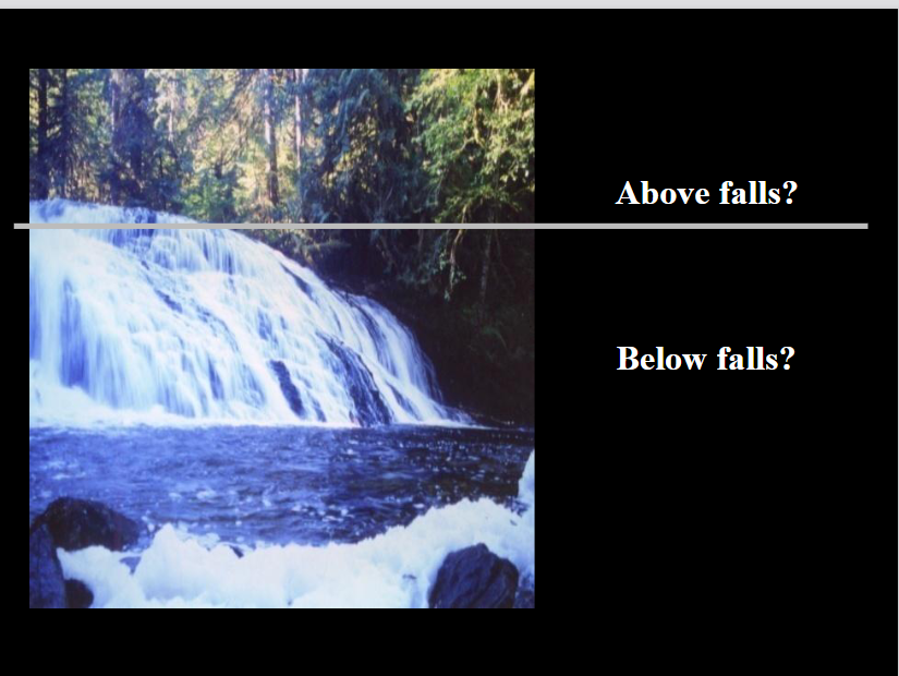
what is this trying to tell me

This slide sets up a natural experiment (control vs. treatment) designed to isolate the exact impact of salmon on the forest floor. It uses a waterfall as a physical barrier to separate an area with salmon from an area without them.

The waterfall acts as a perfect ecological control group. Everything above the falls represents a standard, unmodified terrestrial forest, while everything below the falls represents a forest receiving a massive marine "upload" of nutrients.

1. The Physical Barrier (The Waterfall)

Waterfalls act as a definitive boundary line for ecosystems because migrating salmon cannot jump over massive falls. This splits the stream and its surrounding forest into two distinct zones:

• Below falls: Salmon have full access to spawn here. Bears actively hunt and leave carcasses in this riparian zone.

• Above falls: A salmon-free zone. The water and the surrounding forest receive zero marine nutrient inputs from salmon.

2. The Research Purpose

By comparing the forest above the falls directly to the forest below the same falls, researchers can eliminate outside variables like local weather, general soil types, or tree species.

This allows scientists to definitively answer questions like:

• Do plants below the falls show a high marine nitrogen signature (\(\delta^{15}\text{N}\)) while plants above the falls stay at a standard land baseline?

• Do the trees below the falls grow faster or larger than the exact same species of trees growing just a few meters away above the falls?

explain

This graph displays the direct results of the waterfall natural experiment, proving that plants growing below the waterfall are heavily enriched with marine nitrogen compared to those above it.

1. The Color-Coded Comparison

The data maps out various plant species (like Ferns, Blueberry, Huckleberry, and Western Hemlock) based on their location along the Clatse River:

• 🔴 Above falls (Red dots): These plants sit at a standard land baseline, with \(\delta^{15}\text{N}\) values ranging between -4 and 0. They receive no salmon nutrients.

• 🟢 Below falls (Green dots): The exact same plant species skyrocket to marine levels, with \(\delta^{15}\text{N}\) values surging between +4 and +8.

2. The Core Finding

There is a massive, clear gap between the red and green data points for every single plant species tested. This isotopic data reveals that up to 80% of the nitrogen in riparian plants below the waterfall is derived directly from salmon nutrients. Without the salmon being uploaded by bears, these plants would have the same low nutrient profile as the ones above the falls.

explain this

This slide explores how salmon nutrients physically alter the plant community structure of the forest floor by changing the quality of the soil.

It draws from a 2003 study by Mathewson, Hocking, and Reimchen published in BMC Ecology.

This presentation details how migrating salmon act as a massive "upload" mechanism, transferring vital marine nutrients from the open ocean directly into naturally nutrient-poor terrestrial forests.

This slide provides the statistical proof showing how the plant community structure changes between the salmon-rich and salmon-free zones at the Clatse River waterfall experiment.

It maps the percentage of ground area covered (% Cover) by different types of indicator plants across multiple research plots. Note that the slide title contains a typo and should read "above and below water falls".

1. Top Graph: High Nutrient Indicator Species (Nitrogen-Rich Soil)

This graph tracks plants that demand high amounts of nutrient fertilizer to survive (like Red Alder or Salmonberry):

• Below Falls (Black Bars): These plants thrive, taking up a significant percentage of the forest floor cover (ranging from 10% to nearly 50% across different plots).

• Above Falls (Grey Bars): Because there are no salmon carcasses to fertilize the soil, these high-demand plants are completely absent or barely visible (0% to 5% cover).

2. Bottom Graph: Low Nutrient Indicator Species (Nitrogen-Poor Soil)

This graph tracks hardy, slow-growing plants adapted to low-nutrient, acidic soils (like Salal or Huckleberry):

• Above Falls (Grey Bars): With zero marine nutrient inputs, these stress-tolerant plants dominate the forest floor, locking down 60% to 80% of the ground cover.

• Below Falls (Black Bars): Because the soil is heavily fertilized, faster-growing species outcompete them, dropping their presence down to under 15% cover.

The Clear Conclusion

The presence of salmon creates a complete structural inversion of the forest ecosystem. Above the falls, the forest is heavily dominated by low-nutrient survivalist shrubs. Below the falls, the marine fertilizer completely shifts the competitive balance, turning the forest floor into a dense carpet of high-nutrient demanding vegetation.

This slide introduces the next logical step in the research project: moving from tracking plant types to measuring the physical growth rate of trees over time using a method called dendrochronology (tree-ring analysis).

1. The Core Scientific Question

• "Does the presence of salmon increase the growth rate of plants?"

• While the previous slides proved that plants below waterfalls absorb salmon nitrogen, scientists now want to prove if that marine fertilizer actually makes the long-lived trees grow faster, thicker, and larger.

2. The Methodology: Tree Coring

The large photo shows a researcher using a specialized hand drill called an increment borer to extract a tiny, non-destructive straw-like sample from a massive, ancient coastal tree.

• The Core Sample (Inset Photo): The smaller image shows the resulting wooden cylinder held in a researcher's hand.

• Reading the Rings: Each line on that cylinder represents one year of the tree’s life.

  • Wide rings indicate years with high growth (plenty of nutrients, water, and sun).

  • Narrow rings indicate lean years with poor growth.

Why This Matters for the Salmon Study

By looking at the rings of ancient trees over hundreds of years, scientists can align the tree ring widths with historical salmon population data. If a decade had massive salmon runs, the trees below the waterfall should show significantly wider growth rings during those exact years compared to the trees above the waterfall.

explain

This graph illustrates research showing that salmon-derived nutrients significantly boost the growth rates of Sitka Spruce trees in coastal British Columbia. By feeding on salmon carcasses left behind by predators like bears, these "salmon trees" grow substantially faster than trees without access to these nutrients.

Key Visual Breakdown

• The X-Axis (Timeline): Tracks the years from 1945 to 2000.

• The Y-Axis (Growth): Measures the Mean Ring Width (mm). Wider tree rings indicate more robust growth during that specific year.

• The Color-Coded Regions: The data is broken down into three geographic zones along the BC coast:

  • Mainland (Blue lines)

  • Haida Gwaii (Green lines)

  • Mid-coast (Red lines)

The Main Findings

• Solid vs. Dashed Lines: For each region, the solid line represents "Salmon trees" (trees near rivers with salmon runs), while the dashed line represents adjacent "Control trees" (trees without access to salmon nutrients).

• The Growth Advantage: Across all three regions and all 55 years, the solid lines consistently sit higher than their matching dashed lines.

• The 40% Metric: As highlighted at the bottom of the graph, there is a 40% increase in yearly growth for salmon trees relative to adjacent control trees.

Why Does This Happen?

When spawning salmon return to coastal rivers, predators (like bears and wolves) drag the carcasses into the surrounding old-growth forests. As the salmon decompose, they release massive amounts of nitrogen and phosphorus directly into the soil. This serves as a powerful fertilizer, driving the stark difference in tree ring widths seen in the data.

what r 2 main findgins?

• 500 Years of Consistent Advantage: For nearly the entire five-century span, "Salmon trees" maintained a significantly higher average ring width than the control trees. This proves that the fertilizing effect of salmon isn't just a short-term boost; it alters forest ecosystems across generations.

• The Convergence at the End (Late 1900s): Notice how the red (Salmon) and blue (Control) lines begin to pinch much closer together toward the year 2000. This visual flattening reflects declining wild salmon returns and shifting ecological conditions in the late 20th century, which gradually erased the historic growth advantage these trees once held.

explain

This slide demonstrates that salmon nutrients support the entire coastal food web, extending far beyond just forest plants to directly feed local birds, insects, and apex predators.

Key Ecological Findings

• Winter Wrens (Birds): An isotopic mixing model reveals that 30–95% of the insects eaten by Winter Wrens are sustained by salmon-derived nutrients. Because food is so abundant, the physical density of these wrens is 50% higher in forest areas below waterfalls where salmon can spawn.

• Coastal Wolves (Mammals): The slide highlights that salmon make up about 20% of the fall diet of wolves. Instead of hunting deer or elk exclusively, wolves adapt their behavior in the autumn to forage for spawning salmon along rivers.

• The Isotopic Chart (\(\delta^{15}\text{N}\) vs. \(\delta^{13}\text{C}\)): The graph at the bottom tracks stable isotopes to trace how salmon nutrients flow into forest invertebrates (insects and arachnids).

  • Organisms higher up on the vertical axis (\(\delta^{15}\text{N}\)) have a much higher concentration of marine-derived nitrogen.

  • Fly maggots and specific spiders/millipedes (marked in the red boxes) score very high on this scale, confirming they are directly feeding on salmon carcasses or preying on insects that do.

The Big Picture

This slide ties together the previous lessons on tree growth: spawning salmon don't just act as a simple fertilizer. They act as a foundational energy source that ripples through the ecosystem, directly determining the population size and diet of everything from tiny flies and spiders to songbirds and wolves.

explain

talk about what each kind of hair says about the bears diets

This slide illustrates how scientists use bear hair samples to reconstruct a bear's seasonal diet throughout the year. Because hair grows continuously over time, it acts like a tape recorder—capturing chemical signatures from the food a bear ate weeks or months prior.

The Mechanism: Dietary Time Travel in a Hair Strand

The diagram at the bottom explains how a single strand of hair maps to different seasons:

• The Root (~Fall Diet): The newest part of the hair closest to the follicle reflects what the bear has eaten recently in the autumn (salmon season).

• The Middle (~Summer Diet): Reflects a mid-season diet of berries, insects, and vegetation.

• The Tip (~Spring Diet): The oldest part of the hair strand reflects what the bear ate just after waking up from hibernation in the spring

Reading the Stable Isotope Scatterplot

The graph plots stable isotopes of Nitrogen (d15n) and Carbon (d13c) found in hair segments, color-coded by the time of year they were grown:

• Blue Dots (Spring): Cluster tightly at the lower left. This represents a terrestrial, plant-heavy diet with low marine nitrogen (d15n), as salmon are not yet running in rivers.

• Green Dots (Mid Summer): Begin to shift slightly upward and to the right as diets diversify.

• Red Dots (Late Fall): Shift dramatically to the upper right corner, showing high concentrations of both d15n and d13c. This signature is the unmistakable chemical fingerprint of a heavy salmon diet.

Why This Matters for the Ecosystem

Bears are the primary drivers of the salmon-nutrient cycles explored in the previous graphs. By catching salmon in the rivers and dragging them into the woods to eat, they discard nutrient-rich leftovers. This isotope data maps exactly when and how much bears rely on this critical resource to fatten up for winter hibernation.

whats the main idea of this

This image shows the abstract of a landmark 2017 scientific paper titled "Diverse Ecological Pathways of Salmon Nutrients Through an Intact Marine-terrestrial Interface" by Thomas E. Reimchen from the University of Victoria.

The main idea of this paper is to quantify exactly how nutrients from spawning salmon move through an undisturbed forest ecosystem, mapping out every stage of the food web from bears to soil, bugs, and plants.

This is the first study to completely map out and measure the exact weights, paths, and percentages of how ocean nutrients cross over to land. It provides a vital ecological baseline that helps conservationists understand how to restore damaged, logged, or over-fished river ecosystems across the Pacific Northwest.

explain

what r 3 ecological roles

This slide serves as the ultimate summary of the "Salmon Forest" research, highlighting how bears act as vital ecological conveyor belts that tie ocean productivity directly to the health of coastal land habitats.

Key Summary Points

• Bears as the Primary Movers: Black and grizzly bears are the single most important species responsible for transferring marine nutrients into North Pacific forests.

• Incredible Individual Impact: A single bear can drag up to 500 salmon into the forest over just a short 6-week spawning window.

• Massive Scale of Nutrients:

  • Along spawning rivers, bears drop an average of 1,000 salmon carcasses per kilometer every single year.

  • Across British Columbia, bears leave behind a staggering 2.4 million kilograms of fish remnants annually.

• The Chemical Footprint: Up to 80% of the nitrogen found in coastal mosses, shrubs, trees, insects, birds, and mammals originates directly from the ocean via salmon.

• Boosted Biodiversity: This massive fertilizer injection radically increases overall plant growth (primary productivity) and species diversity in watersheds that have healthy populations of both salmon and bears.

Defining Key Ecological Roles

The slide concludes by classifying how these animals function within the ecosystem:

• Salmon are a keystone species relative to trees (their presence drastically alters the plant community).

• Salmon are a dominant species relative to bears (they provide a massive, foundational biomass for the bears' diet).

• Bears are a keystone species (without them to drag the fish out of the water, the ocean nutrients would never reach the deep forest floor).

whats the main idea of this paper

This image shows the abstract of a critical year 2000 scientific study published in Fisheries titled "An Estimation of Historic and Current Levels of Salmon Production in the Northeast Pacific Ecosystem: Evidence of a Nutrient Deficit in the Freshwater Systems of the Pacific Northwest" by Ted Gresh, Jim Lichatowich, and Peter Schoonmaker.

The main idea of this paper is that the Pacific Northwest is suffering from a massive "nutrient deficit" because modern salmon returns are only a tiny fraction of what they were historically, severely damaging the freshwater ecosystems that depend on them.

The authors conclude that this severe nutrient deficit is a primary indicator of ecosystem failure. It creates a devastating feedback loop: because the rivers lack the nutrients from decomposing salmon, the overall productivity and biodiversity of the watershed drop. This degraded habitat makes it even harder for new generations of salmon to survive, further diminishing the possibility of the salmon population ever recovering to self-sustaining levels.

1. "Downloading" (Land to Ocean)

• The top grey arrow represents the standard, passive direction of gravity.

• Rainfall, weathering, and river nutrients naturally wash off the land and flow down into the ocean.

2. "Uploading" (Ocean to Land)

• The large middle arrow represents the active, biological reversal of this process.

• Marine life acts as an ecological pump, forcing energy and rich marine nutrients back up onto the land, completely defying gravity.

3. The Contributors (The Sub-Arrows)

The smaller arrows at the bottom rank the biological engines driving this "upload":

• Salmon: By far the largest arrow, representing the massive biomass of fish migrating upstream to spawn and fertilize the forest floor.

• Bears & Wolves: The vectors that physically move that salmon biomass out of the water and deep into the woods.

• Seabird Guano, Herring, Kelp, & Intertidal Invertebrates: Other vital marine pathways that deposit ocean-derived nutrients onto coastal shorelines, islands, and nesting grounds.

The Big Picture

While geological forces naturally pull nutrients down into the sea ("downloading"), it is wildlife—led heavily by salmon and bears—that actively "uploads" those nutrients back to sustain the old-growth forests.