SOCI 328 Midterm 3
 Call Kai
 Learn
 Practice Test
 Spaced Repetition
 Match
 Flashcards
 Knowt Play
1/32

There's no tags or description
Looks like no tags are added yet.
33 Terms
Three aspects of association between two categorical variables
Direction of association (contingency table)
Strength of association (Carmer’s V, Kendall’s tau-b)
Statistical significance of association (Chi-squared test of significance)
Contingency table
table that displays the number of observations observed at all the combinations of possible outcomes for the two variables
AKA cross-tabulations, two-way tables, crosstabs
Percentages calculated going across rows, compared percentages vertically

Marginal distributions
row totals and column totals that are considered together; frequency distributions for two variables
Row percentage
percentage of total row that pertains to the column
Cramers’s V
a measure of the strength of an association between two categorical variables
Can be used for bivariate and multivariate nominal variables
Doesn’t consider ordinal aspects of variables
Ranges from 0 (no association) to 1 (perfect association)
Kendall’s Tau-b
measure of strength of association between two ordinal variables, indicating direction of association unlike Cramer’s V
Ranges from low of -1 (perfect negative association) through 0 (no association) to a high of 1 (perfect positive association)
Observed count
number of observations in the sample that belong in each associative category (ie. in each cell)
Counts of what you actually found in your sample
Expected count
number of observations you would expect to find if there was no association between the two variables in the population
Standardizes row percentages so they are the same across all rows

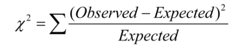
Chi-squared
test statistic that calculates the statistical significance of association found; calculates the likelihood that the association is found by chance given the null hypothesis is true (ie. p-value)
If there is little difference between observed and expected values, indicates that Chi-squared value is small and the effect of the variables on each other is small since there is little difference from no effect
Data assumptions for Chi-squared test
No more than 20 of the expected counts are less than 5
All individual expected counts are 1 or greater
Must be enough expected counts in the cells for test statistic to work
IN a 2×2 table all four expected counts should be 5 or greater
Statistical vs. Practical significance
Small p-value does not necessarily imply a statistical significance due to the effects of large sample size
Larger samples produce smaller p-values for weak associations so its possible to have weak practical significance but appears statistical significance due to large sample size

Test of Significance for Kendal Tau-B
Test of significance for an ordinal x ordinal variable
More discriminating than Chi-squared test due to consideration of order
Tau-b less effective when there is more than one trend in association
Numerical by Numerical association techniques
Scatterplot
Pearson’s r
OLS regression line
Spearman’s rho
Scatterplot
visually depicts the association between two numerical variables, where each case in the data appears as a point on the plot
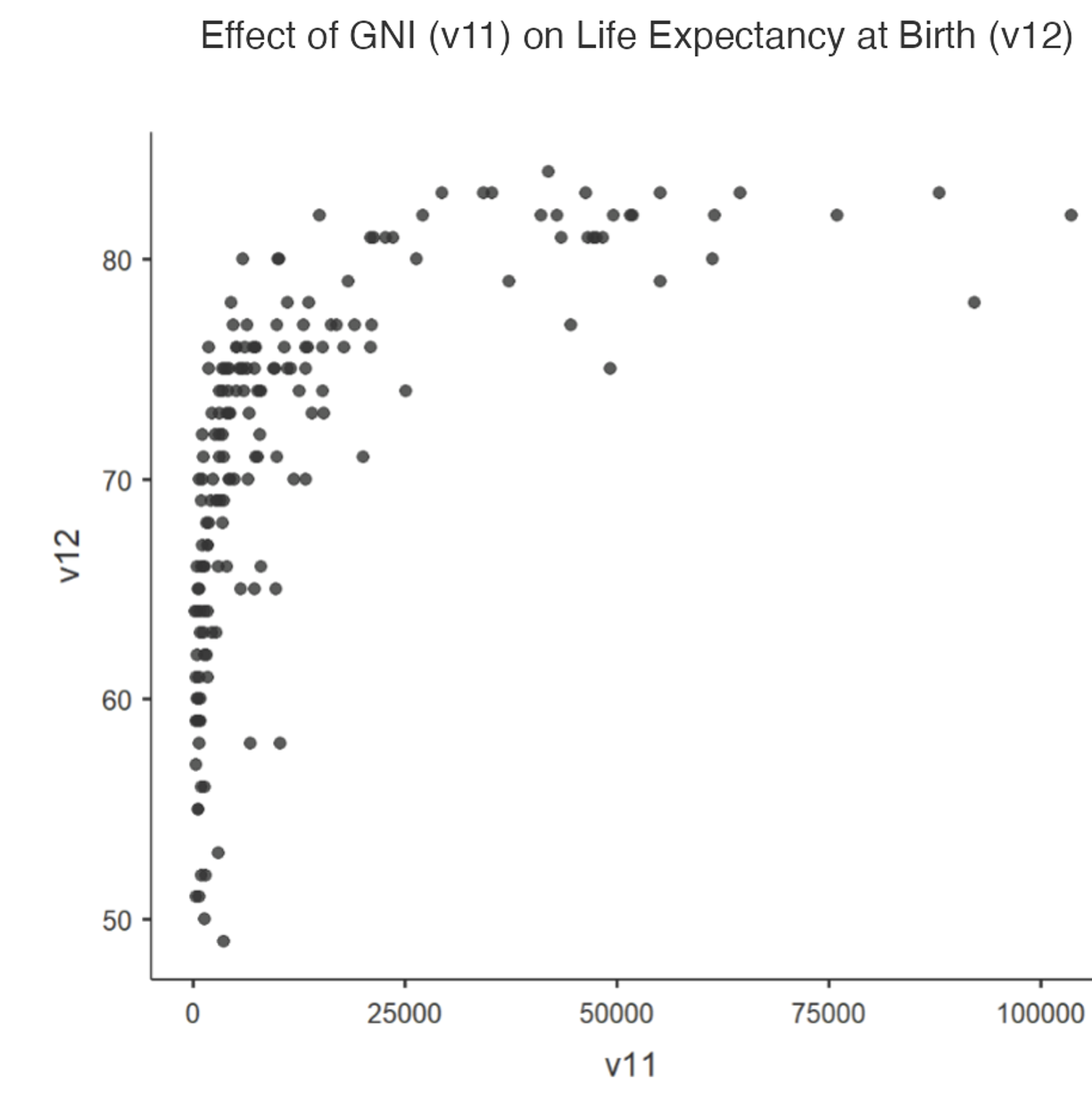
Patterns in Scatterplots
Direction of association (positive, negative)
Strength of association (very weak, weak, moderate, strong, very strong)
Linear or curvilinear
Are there outliers?
LOWESS curve
Polynomial function that is to fit to the data in a scatterplot using a weighted least squares procedure
Determines whether association has significant nonlinearity
Pearson’s r
statistic that measures the direction and strength of a linear association between two numerical variables
Can interpret a curvilinear association into a linear association by transforming variable with a root or log
Characteristics of Pearson’s R
R is positive when association is positive; r is negative when association is negative; r = 0 represents no linear association
R= 1 is perfect positive linear association
R = -1 is a perfect negative linear association
Magnitude of r corresponds with strength of association
R makes no distinction between independent and dependent variables
R only describes linear associations, not curvilinear associations
Is not resistant to outliers due to reliance of use on mean and standard deviation
Each points in each quadrants are added and divided by number of values
If majority of points are in top right and bottom left quadrants, Pearson’s r will be positive thus making it a positive association
Multiplying positive by positive or negative by negative in these quadrants creates a positive number
Closer points are to the blue line, the larger Pearson’s r will get ➔ indicates a stronger relationship
If you multiply numbers closer to blue line, number will be bigger than if it is closer to 0, the x and y axis
Transformign variables
Can transform variables with root or log if association is nonlinear
Square root if skewed to right
Log if skewed to left
Assumptions of Pearson’s R
- Both variables are roughly symmetric
- Association between variables is linear
- There are no inordinately influential outliers
Hypotheses of Test of Significance for Pearson’s r
o H0: r equals 0 in the population
o Ha: r does not equal 0 in the population
Spearman’s rho
assesses direction and strength of an association between two numerical data by replacing actual data values with ranks and executes a Pearson’s correlation on the ranked area
Can be used when original association is curvilinear
More resistant to outliers than Pearson’s R
Loses information regarding actual values of points
Better to use Pearson’s r if relationship is linear
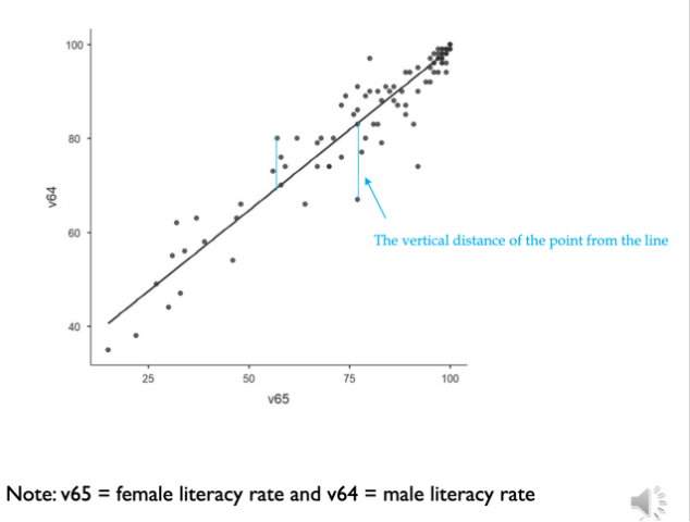
OLS Regression Line
straight line that represents that pattern of points to summarize the nature of the linear association between two variables
Minimizes the sum of the squared residuals
Beta
standardized regression coefficient of b
R squared
coefficient of determination which is the proportion of total variability in Y that can be attributed to X
Ie. how well the line fits to the data set while r is just direction of the relationship
Measures strength of association

Anscombe’s quartet
Regression results for graph may note necessarily reflect the validity of the scatter plot
