intro to stats: unit 2 overview

Topics: Categorical vs quantitative variables Individual, sample, population Displaying data - drawing and interpreting bar graphs, pie charts, dotplots, stem-and-leaf plots, histograms, box plots Measures of center - mean, median, mode Measures of spread/variability - range, IQR, standard deviation Describing and comparing distributions - SCVO (shape, center, variability, outliers) Skewness - effects on mean/median and IQR, calculating outliers

Categorical variable

A characteristic that places an individual into one of several groups, categories, or labels

Quantitative variable

A variable that can be measured and expressed numerically, allowing for mathematical operations and statistical analysis.

Individual

A single entity or unit that is being studied, observed, or measured in statistical analysis or research.

Population

The entire group of individuals about which information and conclusions are desired. Example: All 1,200 students enrolled at a high school.

Sample

A subset of individuals selected from a larger group from which data is collected. Example: A randomly selected group of 60 students chosen from the high school

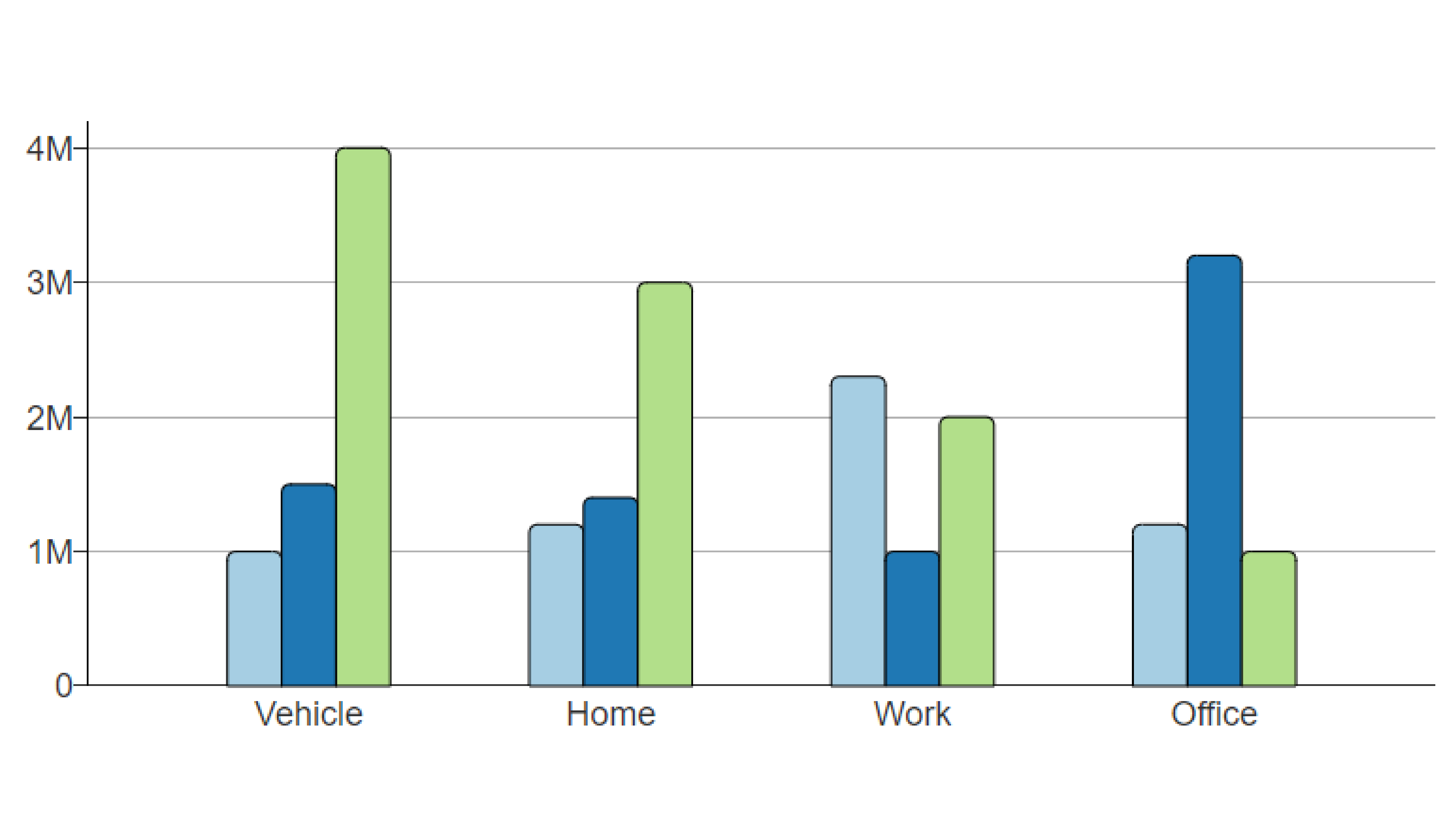
Bar Graph

A visual display for categorical data where separated rectangular bars indicate the frequency or relative frequency of each category. It helps in comparing different categories visually, making it easier to identify trends or differences in the data. . Example: A chart showing the counts of students who commute by car, bus, bicycle, or walking.

Pie Chart

A circular statistical graphic divided into slices, each representing a category's proportion of the whole (100%). Example: A chart showing the percentage breakdown of a school's population by grade level.

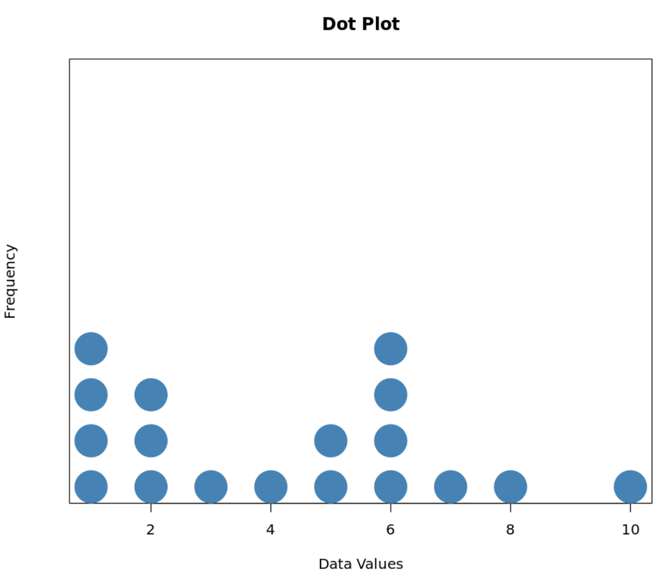
Dotplot

A quantitative display in which each data point is stacked as a dot above its corresponding value along a number line. Example: Stacking dots above numbers from 0 to 5 to show how many pets each surveyed classmate owns.

Stem-and-leaf plot

A quantitative display that separates each value into a leading digit (stem) and a trailing digit (leaf) to show distribution shape while retaining exact values. Example: A stem of 7 and leaf of 4 representing a test score of 74.

Histogram

A display for continuous quantitative data that groups values into adjacent, equal-width intervals with bar heights showing frequencies. Example: A graph showing the number of students who studied between 0 and 10 hours, 10 and 20 hours, and 20 and 30 hours.

Boxplot

A visual representation of the five-number summary: minimum, first quartile (Q1), median, third quartile (Q3), and maximum. Example: A display illustrating the spread of exam scores from a minimum of 52 to a maximum of 98.

Mean

The arithmetic average of a quantitative dataset, found by summing all values and dividing by the total count: Example: For test scores 80, 85, and 90, the mean is 80+85+90 / 3= 85

Median

The middle value in an ordered set of quantitative observations that divides the data into two equal halves. Example: In the ordered list 3,5,8,11,14, the median is 8.

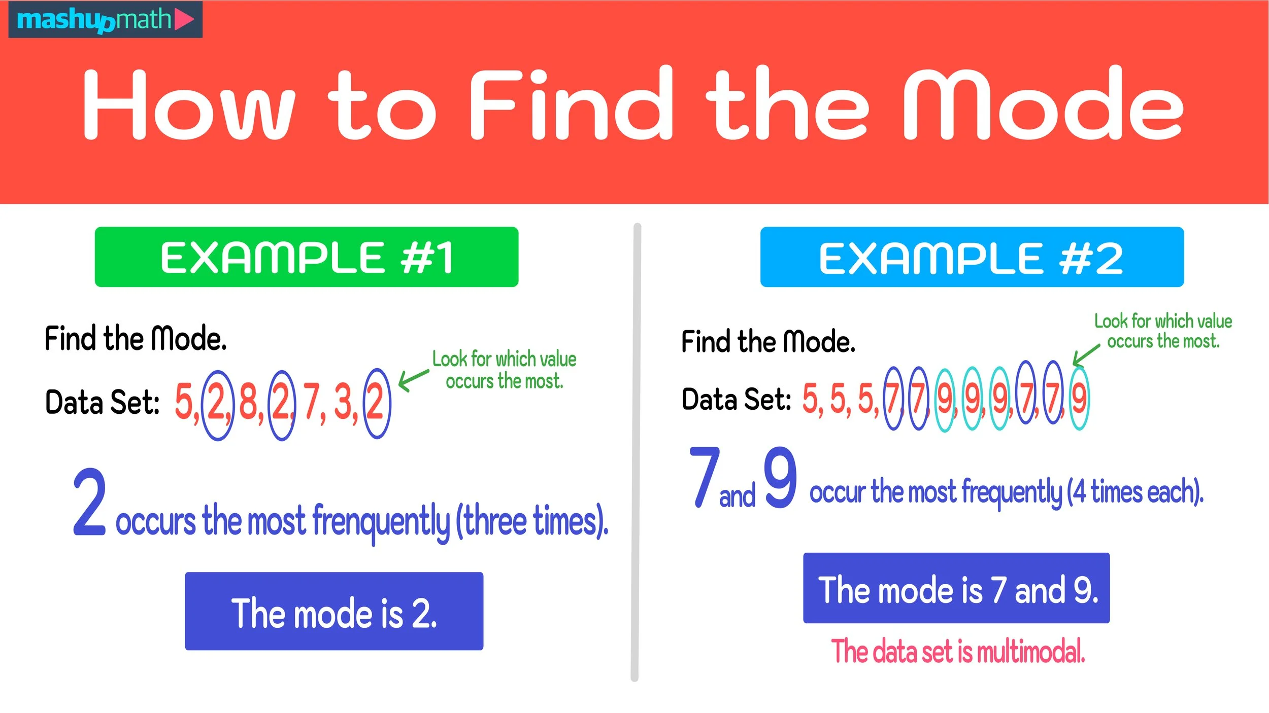
Mode

The data value, class interval, or category that occurs most frequently in a distribution. Example: In the dataset 4,6,6,7,9 the mode is 6.

Range

The difference between the maximum and minimum values in a quantitative dataset: Range=Maximum−Minimum

Example: If the highest test score is 96 and the lowest is 58, the range is 96−58=38.

Interquartile Range (IQR)

The spread of the middle 50% of an ordered dataset, calculated as IQR=Q3−Q1. Example: If the third quartile is 88 and the first quartile is 70, then IQR=88−70=18.

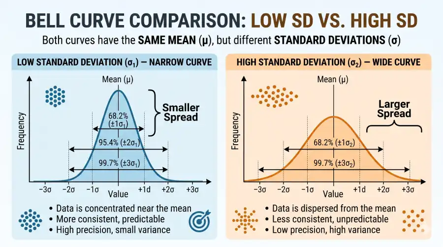
Standard deviation ( s )

A measure of spread describing the typical distance of observations from their mean: Example: A set of quiz scores with s=2 points indicates much closer clustering around the average than a set with s=9 points.

SCVO framework

The four essential characteristics used to describe and compare quantitative distributions are: Shape, Center, Variability, and Outliers. Example: Describing a distribution as unimodal and right-skewed, centered at a median of 14, with an IQR of 6, and an outlier at 35.

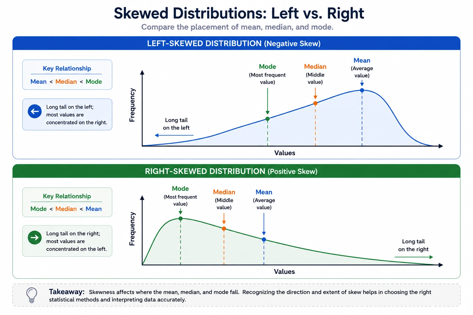
Effect of right-skewness on center

A distribution with a long right tail pulls the mean upward, making it greater than the median (Mean>Median). Example: In salary data where a few executives earn millions, the mean salary is pulled much higher than the median salary.

Effect of left-skewness on center

A distribution with a long left tail pulls the mean downward, making it less than the median (Mean<Median). Example: On an easy exam where most students score near 95 but a few score near 30, the mean is dragged below the median.

Outlier detection rule (1.5×IQR rule)

A rule identifying any observation as an outlier if it falls below Q1−1.5×IQR or above Q3​+1.5×IQR. Ex. With Q1=40 and IQR=10, any score below 40−1.5(10)=25 is flagged as an outlier.

Resistant summary statistics

Summary measures that are not substantially influenced by extreme values or skewness, namely the median and IQR. Example: If an extreme score of 1,000 is introduced into a set of standard exam grades, the median and IQR remain stable while the mean spikes.