The Beast of Bias + Mediation
 Call Kai
 Learn
 Practice Test
 Spaced Repetition
 Match
 Flashcards
 Knowt Play
1/19

There's no tags or description
Looks like no tags are added yet.
20 Terms
How do we detect outliers? (2)
1. Graphs, histograms, scatterplots (less helpful with several predictors)
2. Standardised residuals

Residual
The difference between an actual observed value and the value predicted by a model.
Standardised residuals
Residuals expressed in standard deviation units.
~ 95% should fall within ±2 and 99% within ±2.5. Absolute values ≥3 suggest outliers.
Influential cases
Observations that substantially affect the fitted linear regression model (e.g., its slope or intercept).
An outlier is not necessarily influential.
Methods of detecting influential cases
DF beta
Cook’s distance
DF beta
Measures how much an individual regression coefficient (b) changes when an observation is removed. Absolute standardised values >1 are concerning.


Cook’s distance
Measures the influence of a single case on the model as a whole.
Absolute values >1 are cause for concern, any larger than 0.5 are likely to be influential.

Key assumptions of the General Linear Model (GLM)
Linearity (straight-line relationships)
Additivity (predictor effects add together)
Spherical errors (homoscedastic + independent errors)

Additivity
The combined effect of predictors equals the sum of their individual effects
Spherical errors
Errors must be independent (uncorrelated) and homoscedastic (constant variance).
Errors vs Residuals
Errors: The true, unobservable difference between an actual outcome and the real population prediction.
Residuals: The observable difference between an actual outcome and your sample model's prediction
Autocorrelation
Autocorrelation happens when errors are correlated with each other (often across time or sequence). It violates the independence assumption.
(That errors for different data points must not be linked or predictable from one another)
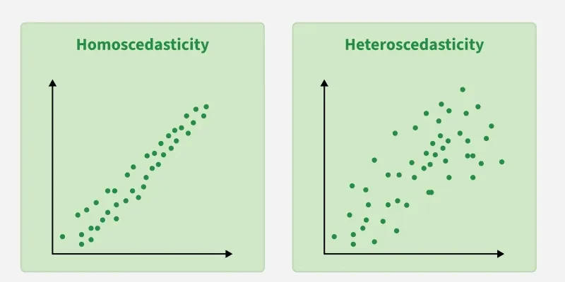
Homoscedasticity vs heteroscedasticity
Homoscedasticity: The error (spread of data) stays the same across all values.
Heteroscedasticity: The error (spread of data) changes as values get bigger or smaller.
Central Limit Theorem (CLT)
The more samples you have, the distribution will closely resemble a normal disturbution regardless of the original population distribution.
Sample size and normality
Large samples generally reduce concerns about non-normality for inference, but do not guarantee normality. In smaller samples, bootstrapping may provide an alternative for estimating uncertainty.
Robust model procedures


Bootstrapping
Used for small samples
Repeatedly resamples observations WITH replacement, recalculating a statistic each time to create an empirical sampling distribution.
picks a number and puts it back in and creates a mean from this. and again and again
Heteroscedasticity-consistent (HC) standard errors
Robust standard errors that adjust for non-constant error variance, improving statistical inference when homoscedasticity is violated. Calculated using a sandwich estimator.
HC3 and HC4 models work best
Mediation
Meditation is when the relationship between a predictor and outcome can be explained by their relationship to a third variable.
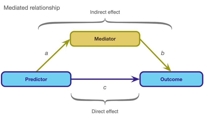
The total effect between a predictor and outcome can be broken down into:
The direct effect: The relationship between the predictor and outcome adjusting for the mediator (path c)
The indirect effect: The relationship between the predictor and outcome via for the mediator (path ab)
Total effect = c + (a x b)
