STATS EXAM 2
 Call Kai
 Learn
 Practice Test
 Spaced Repetition
 Match
 Flashcards
 Knowt Play
1/37

There's no tags or description
Looks like no tags are added yet.
38 Terms
Sample surveys
use randomization to get representative sample
A SURVEY NEVER ESTABLISHES CAUSATION
voluntary response bias
when study or survey participants are self-selected volunteers rather than randomly chosen by the researcher
open to everyone
ex: a poster advertising a survey with a link
nonresponse bias
the researcher selects a random sample, but specific chosen individuals decline to answer or cannot be reached
simple random sample (SRS)
a subset size n is chosen from a larger population size N such that every possible combo of n individuals has an equal probability of being selected
Stratified sample
researcher divides a total population into smaller, non-overlapping, and homogeneous subgroups called strata based on shared characteristics (eg., age, income, education lvl, location)
multistage sample
selects a sample in progressive, smaller hierachical steps or stages
instead of sampling the entire population at once, researcher break the selection down into hierarchical units:
PSUS
—>SSUs
USUs
cluster sample
population is divided into seperate, non-overlapping groups (clusters), and a random sample of those clusters is selected for study
ex: want to survey 10th graders across all of NYC, so you use the schools as natural clusters, list every single school in NYC, then randomly pick 10, and collect data
systematic sample
researchers select members from a larger population by picking a random starting point then choosing subsequent members a t a fixed, regular interval
there are 1,000 customers, and your desired n is 100 —> 1,0000/100=10 —> pick a random starting point (ex: 7)—> choose 7th customer on the list, then every 10th customer after that until you reach 100 total participants
Observational studies
researchers observe subjects W/O assigning treatments.
can show association but NOT CAUSATION
experimental studies
researchers can randomly assign treatments to subjects
CAN establish causation
experimental design terms
experimental units (e.g., ppl, plants, or anything that is being tested)
factor
levels
response variable
lurking variables
confounding variables
experimental units
factors
the explanatory variable manipulated by the researcher
ex: a dosage of something, or the diet someone is given
test example: the factor in the pizza delivery question is calling the customer
levels
the specific values or categories of a factor
ex: 0mg, 50mg, 100mg
test example: the level in the pizza delivery question is whether the customer was called or not
lurking variables
an unmeasured variable that is not part of the study and affects both X and , altering or distorting the perceived relationship between them
usually tied to observational studies
ex: a patients age or weight
confounding variables
an outside or “third” variable that correlates with both the independent variable (the cause) and the dependent variable (the effect)
usually tied to experimental studies
lurking vs. confounding
a lurking variable affects both X and Y in an observational study WHEREAS a confounding variables effects on the response cannot be separated from the factors effects in an experiment
4 principles of experimental design
control
randomize
replicate
block (if needed)
Normal model conditions (proportions)
randomization
10% condition
success/failure condition
central limit theorem (CLT)
even if a population is skewed, the sampling distribution of the sample mean (y-bar) becomes approximately Normal as n increases (usually n>_ 30)
when to use CLT
the problem gives you a mean, a standard deviation, and asks for the probability, percentage, or cutoff value (percentile/IQR)
CLT Model
y-bar ~ N (M, o/√n)
Mean of sampling distribution
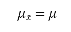
standard deviation of sampling distribution
SD(y-bar)=o/√n
USE WHEN: you need to find how much the average of a random sample (y-bar) is expected to vary from the true population avg (M)
confidence intervals for proportions (when to use)
youre estimating a population percentage/proportion, and the problem gives a sample size (n), and either a sample percentage (p^) or count of successes (x)
CI for proportion formulas
standard error
margin of error
intervals (lower and upper bound)
Sample size (n) for a desired Margin of Error (ME)
use when the question asks “how many…” or “what sample size is needed…” to get a specific ME (e.g. “within 3%”)
Sample size (n) for a desired Margin of Error (ME) FORMULA
n=((z*)²xp^q^)/ME²
if no p^ is given USE p^=0.05
Confidence intervals for means
use when you are estimating a population average/mean, and the problem gives a sample size (n), sample mean (y-bar), and sample SD (s)
knowing when to use t* vs z*
when you only have the SAMPLE SD (s), and not the true population (o), you must use t*
Formulas for calculating CI for Means
degrees of freedom (df)= n-1
standard error: SE(y-bar)=s/√n
bounds: sample mean (y-bar) ± t*(SE)
HOW TO FIND t* in CRUNCH
stat —> calc —> T —> click between —> enter df —> enter the CI as a decimal (eg: 90% CI —> 0.90) in the box after = —> compute
what does it mean if a CI increases
the interval gets wider, and ME increases
what does it mean if the sample size (n) increases
the interval gets narrower, and ME goes down
checking a claim w/ a CI
check if the claimed number is inside your interval: inside = plausible (no difference), outside = evidence of a real difference
when do you know if a question is asking about hypothesis testing & p-values
question asks you to test a claim, asks “is there convincing evidence…” or gives you a significance level (ex: a=0.05) and a P-value
hypotheses
H0= no change
Ha=
“changed”, “differed”, “not equal” —> two-tailed (≠)
“less than”, “decreased”, “lower” —> left tailed (<)
“greater than”, “increased”, “improved” —> right tailed (>)
how to make your final decisions w/ hypotheses
COMPARE P TO α
if P < α —> REJECT H0, results are statistically significant, and there IS convincing evidence for Ha
if P >_ α —> FAIL to reject H0, results are NOT statistically signif, and there is NOT enough evidence to support Ha