ECON 2310 pre-exam 1.1
 Call Kai
 Learn
 Practice Test
 Spaced Repetition
 Match
 Flashcards
 Knowt Play
1/136

Earn XP
Description and Tags
good luck!
137 Terms
Economics suggests important relationships, often with policy implications, but virtually never suggests
quantitative magnitudes of causal effects
using data to measure causal effects - how do we get this data?
(Ideal) Randomized controlled experiment
– cost, cooperation, ethical
randomized controlled experiment
two groups, randomly assign which one is experimental and control, compare both to estimate the causal effect
examples of other sources of data
more commonly we have observational data
survey, administrative records, historical records, mortgage applications, etc.
-- cross-sectional (i), time series (t), panel data (i,t)
issues with observational data
“treatment” is not random
-- unobserved heterogeneity
prediction
use the value of some variables to make a statement of another variable
forecast
a prediction about the value of a variable in the future
A good prediction does not require
a causal relationship
• Modern machine learning methods with a large number of predictors
• Forecast with time series data
joint distribution
Random variables X and Z have a joint distribution
The covariance is a measure of the linear association between X and Z
– cov(X,Z) > 0 means a positive relation between X and Z
If X and Z are independently distributed, then cov(X,Z)
cov(X,Z) = 0 (but not vice versa!!)
linear association

The correlation coefficient measures
linear association
conditional expectations

conditional variance is the
variance of the conditional distribution
simple random sampling
Choose an individual (district, entity) at random from the population
before sample selection, Y is random because individual selected is random
Once selected Y is observed and therefore a non-random value
iid
individually and independently distributed
Because individuals #1 and #2 are selected at random, the value of Y1 has no information content for Y2. Thus:
– Y1 and Y2 are independently distributed
– Y1 and Y2 come from the same distribution, that is, Y1, Y2 are identically distributed
– More generally, under simple random sampling, {Yi}, i = 1,…, n, are i.i.d.
iid allows
This framework allows rigorous statistical inferences about moments of population distributions using a sample of data from that population …
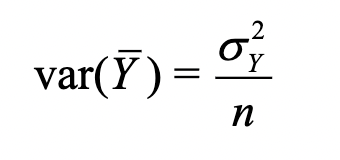
breaking down mean

breaking down variance
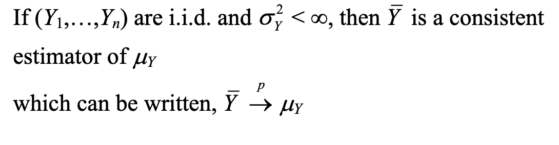
An estimator is consistent if
the probability that its falls within an interval of the true population value approaches 1 as the sample size increases.
Law of Large Numbers
Central Limit Theorem
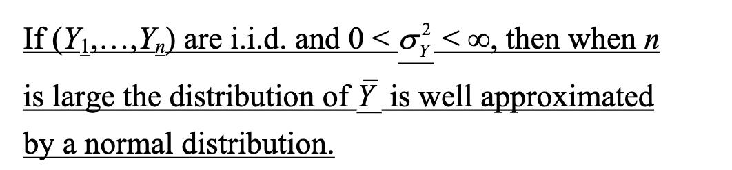
CLT - larger n the better

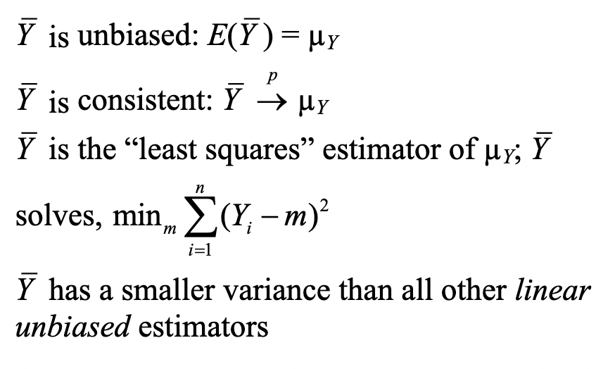
why use sample average
The hypothesis testing problem: .
make a provisional decision, based on the evidence at hand, whether a null hypothesis is true, or instead that some alternative hypothesis is true
1 vs 2 sided

test statistic

anatomy of test statistic

estimation of variance

significance level
probability of incorrectly rejecting the null hypothesis when it is true.
– Pre-specified, e.g., 5%.
For a two-sided hypothesis testing with the t-statistic, Pr(|t|>cv) = significance level
critical value
value of the statistic for which the test rejects the null hypothesis at the given significance level.
p value
Probability of drawing a statistic at least as adverse to the null hypothesis as the value you actually computed in your sample, assuming that the null hypothesis is true.
calculating p value based on Y mean

Suppose that, in your sample of recent college graduates, the average wage is $22.64. The p value is
the probability of observing a value of 𝑌(bar) at least as different from $20 (population mean under null hypothesis) as the observed value of $22.64 by pure random sampling variation, assuming that the null hypothesis is true.
from wage example, if p value is small
If p-value is small (0.1%), then it is very unlikely that this sample would have been drawn if the null hypothesis is true
→ null hypothesis is not true.
from wage example, if p value is large
If p-value is large (40%), then it is quite likely that the observed sample average of $22.64 could have arisen just by random sampling variation if the null hypothesis is true
→ evidence against the null hypothesis is weak, and it is reasonable not to reject the null hypothesis.
p value graphically

for large n the p value is the probability that

math on adding estimated standard error into p value test statistic
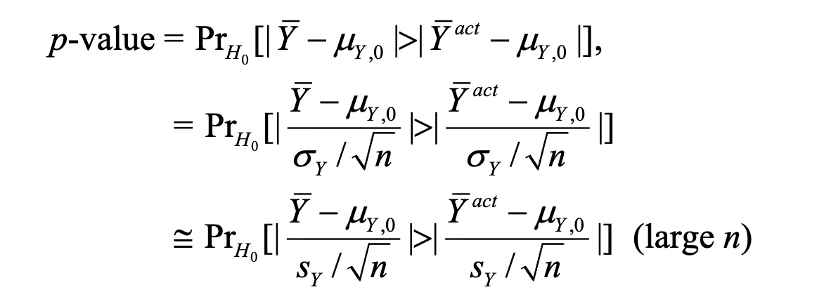
final p value with estimated standard error

link between p value and significance level
The significance level is prespecified. For example, if the prespecified significance level is 5%, you reject the null hypothesis if |t| ≥1.96
equivalently, you reject if p ≤ 0.05
Often, it is better to communicate the p-value than
simply whether a test rejects or not – the p-value contains more information than the “yes/no” statement about whether the test rejects.
A 95% confidence interval for Y bar is
an interval that contains the true value of Y mew in 95% of repeated samples.
Digression: What is random in a confidence interval?
The values of Y1,…,Yn and thus any functions of them – including the confidence interval.
The confidence interval will differ from
one sample to the next. The population parameter, Y mew, is not random, we just don’t know it.
A 95% confidence interval can always be constructed as
the set of values of Y mew not rejected by a hypothesis test with a 5% significance level.

population linear regression model

anatomy of population regression model

B0 B1 and u

population regression line notation - STR

The population objects (“parameters”) B0 and B1 are
unknown; to draw inferences about these unknown parameters we must collect relevant data.
simple random sampling in regression
Choose n entities at random from the population of interest, and observe (record) X and Y for each entity
Simple random sampling implies that
{(Xi, Yi)}, i = 1,…, n, are independently and identically distributed (i.i.d.).
Note: (Xi, Yi) are distributed independently of (Xj, Yj) for different observations i and j.
How do we estimate B0 and B1 from data?
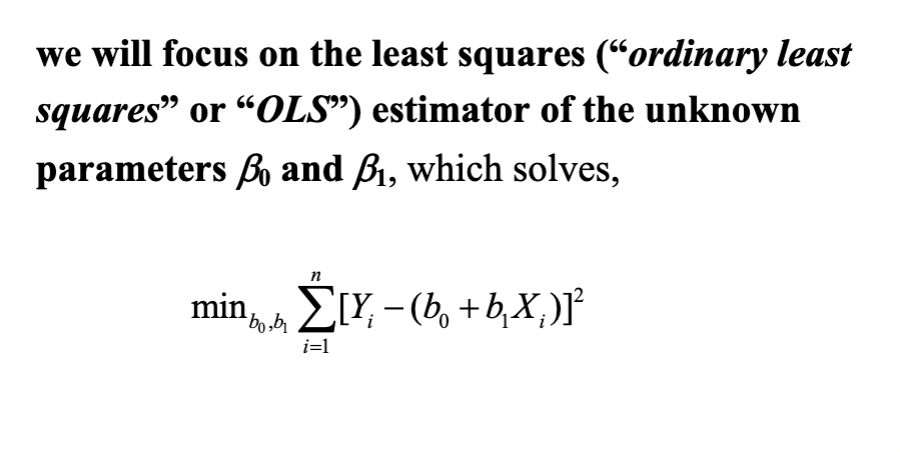
OLS estimator solves

The OLS estimator minimizes the
average squared difference between the actual values of Yi and the prediction (predicted value) based on the estimated line.
• This minimization problem can be solved using calculus
• The result is the OLS estimators of B0 and B1.
OLS estimator B1

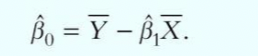
OLS estimator B0
estimated predicted values of Yi

estimated residuals of ui.


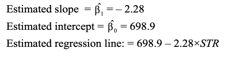
estimates based on equation
matrix representation
We can write the data in matrix and the OLS estimator can be easily obtained with matrix calculation. This requires knowledge from matrix algebra. Computing packages also use matrix calculations.

What will Yi and ui be here?

predicted value - plug in test score
residual - plug in actual value to observe gap between predicted and actual
How do we see how a regression line fits?
R2 or standard error
R2
The regression R2 measures the fraction of the variance of Y that is explained by X; it is unitless and ranges between zero (no fit) and one (perfect fit)
standard error regression
• The standard error of the regression measures the fit – the typical size of a regression residual – in the units of Y.
explained sum of squares

total sum of squares

sum of squared residuals
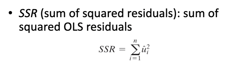
two expressions of R2 are equivalent, or

Notes on R2

standard error of regression
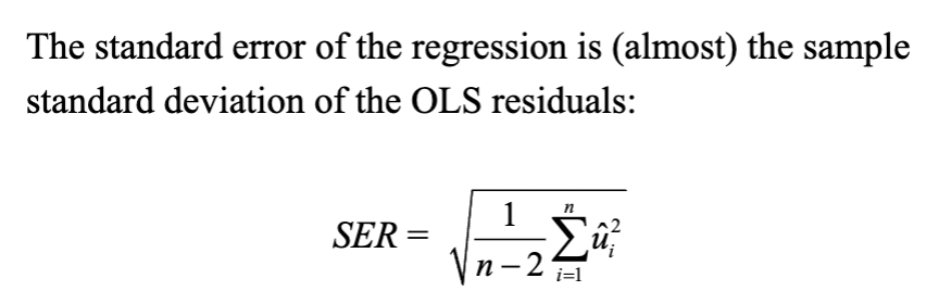
notes on SER

root mean squared error

OLS is a generalization of sample average

how to use OLS estimates?
Prediction: use the OLS regression line directly
• Interpretation: we should examine the model more carefully before drawing a causal relationship
looping in slope into regressions

interpretation of estimated slope and intercept, test scores

assumptions on previous estimates/slope

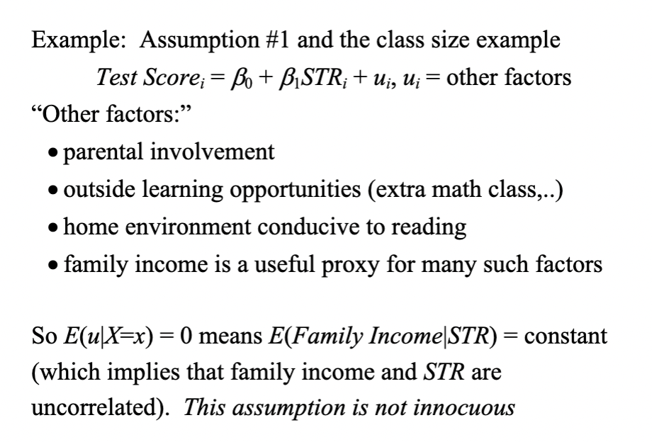
Least Squares Assumptions for Causal Inference: the conditional distribution of ui given Xi has mean
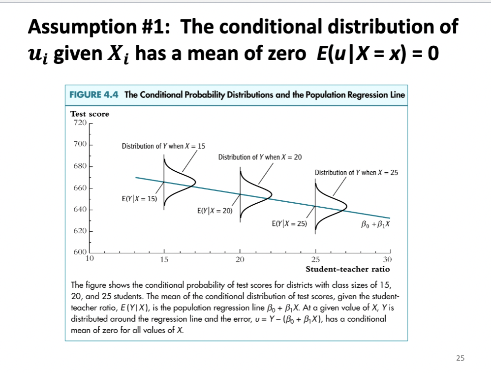
assumption 1: explaining conditional expectation E[ui|Xi]
assumption 2 - (Xi, Yi) are

This arises automatically if the entity (individual, district) is sampled by simple random sampling.
• The main place we will encounter non-i.i.d. sampling is when data are recorded over time (time series data) – this will introduce some extra complications.
Assumption #3: Large outliers are

Moments describe a distribution's shape: the first is the mean, the second relates to variance, the third to skewness, and the fourth to kurtosis, or how heavy the tails are. Requiring a finite fourth moment means the tails can't be so fat that extreme observations show up too often. It's a way of saying "outliers are rare enough that they don't dominate the sample."
Why OLS needs it
The assumption isn't needed for unbiasedness. It matters for the large-sample results:
Consistency of the variance estimates. OLS standard errors rely on sample variances and covariances converging to their population values. The sample variance of X is an average of squared deviations, and for a law of large numbers to apply to that average, the variance of (X − μ)² must be finite. That variance involves E[(X − μ)⁴], which is the fourth moment.
The CLT for the slope. The asymptotic normality of β̂₁ comes from a CLT applied to terms like (Xᵢ − μₓ)uᵢ. That requires this product to have finite variance, and finite fourth moments of X and u guarantee it (via Cauchy-Schwarz). Heteroskedasticity-robust standard errors need this too.
least squares assumptions role 1
Role 1: mathematical. If assumptions hold, then, in large samples, OLS estimators are consistent and have sampling distributions that are normal
→ underpin methods for testing hypotheses and constructing CI
least squares assumptions role 2
Role 2: organize circumstances that pose difficulties for OLS estimation of causal effect 𝛽1
– Assumption #1 is most important to consider in practice
– Assumption #2 holds plausibly in cross-sectional data, the independence assumption is inappropriate for panel and time series data
– Assumption #3 reminds us that OLS can be sensitive to large outliers
Because OLS estimators are calculated using a random sample,
est𝛽0 and est𝛽1 are random variables that take on different values from one sample to the next.
• Probability of these different values is summarized in their sampling distributions.


Proof estimate B1 is unbiased

algebra of sampling distribution of estimate B1

expanding on B1 hat algebra

expanding on B1 hat algebra p2

simplify formula

building on simplified B1 hat formula

adding in expectation of ui over Xi

Now we show the large-sample normal approximation to the limiting distribution of B1 hat
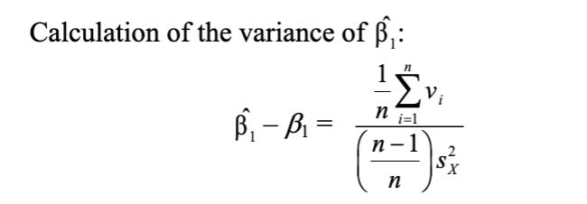
this calculation is simplified by supposing that n is large

Under the three Least Squares Assumptions

estimator of variance of B1 hat

for above card