UCLA STATS 101A Final

Conditions to interpret Confidence Interval for difference between means

1. Independence of groups, observations: samples from groups, observations should be independent of each other

   • eg. Groups are dependent if you surveyed females and males in the SAME household

2. Random sampling

3. Normality: sampling distribution of difference between two means should be normal

   • If population dist is normal, this will be normal. Otherwise, need the Central Limit Theorem

4. Equal variances: CI can be more precise if this is true, will be approximated if not

Confidence Levels, Intervals

• Lower confidence level → narrower confidence interval

• Width is determined by CL, pop variability, variability of estimated statistic

• If you were to generate many CI’s, CL% of the intervals will contain the population parameter

  • CI’s say NOTHING about sample statistics

  • CL% of ALL possible intervals based on same sample size will contain the population parameter

• BEFORE taking a random sample, the probability that your CI contains the parameter is CL%

• Valid with:

  • random sample

  • large sample size (CLT)

  • independent observations

• smallest at the mean (xbar)

Standard Error

• Typical “distance” of statistic from parameter, how it varies sample to sample

• Standard deviation of a sampling distribution

• Becomes smaller with larger samples or small standard deviation

• Included as a margin of error in confidence intervals, with tuning parameters based on CL

Sampling distribution

• Distribution of statistics, or theoretical samples

• Its standard deviation is the Standard Error

Central Limit Theorem

• Shape of the sampling distribution becomes normal with larger samples, NOT the population OR the sample itself

null hypothesis

assumed to be true when calculating the p-value

significance level

probability of rejecting the null hypothesis when it is true

probability of making a Type I error

alpha = 1 - confidence level

p-value

• probability, when null hypothesis is true, that a random sample will generate a test statistic as extreme or more than observed value

  • not the probability that the null hypothesis is T/F (it’s assumed true)

  • not the probability that results might be due to chance

• if H_0 is true, follows a uniform distribution on [0,1]

• computed based on sampling distribution of test statistic where H_0 is true

alternative hypothesis

• what is left after rejecting the null, but not “accepted”

hypothesis tests are statements about

parameters

t-distribution

• used when population standard deviation (and therefore SE) is unknown (which is most of the time)

• thicker tails than normal dist, more variability to account for extra distortion

• part of the tuning parameter for margin of error in a mean confidence interval

t-statistic

• test statistic used for the mean, slope of a regression line

• how many SEs away the tested statistic is from the null statistic

• when H_0 is correct:

  • this will be close to 0

  • its sampling distribution will be the t-distribution

bias in estimators

• check center of estimator sampling distribution; how far off is it from the parameter?

precision in estimators

• check standard deviation of sampling distribution (SE); how wide is it?

interpreting linear model parameters

• linear models make predictions about averages

ex. Test scores in Des Moines are, on average, 8 points below those in Cedar Rapids.

z-score

how many SDs an observation is from the mean

trend component of model validity

does the model fit the trend?

residual plot should have no trend, flat

slope and intercept will be biased

constant variance component of model validity

is variance constant across all x?

residual plot should be flat, no megaphone/fan shape

scale-location plot should NOT have an increasing/decreasing trend

all inference tools invalid

normal component of model validity

are errors normally distributed?

QQ plot points should fall in a straight line, slight variation at ends is acceptable

inaccurate prediction intervals; symmetric interval won’t work

unbiased intercept, slope

for large sample size, good p-values, confidence intervals

independence component of model validity

are errors independent?

shouldn’t see patterns across timestamp/order observed (plot residuals by order taken)

all inference tools invalid

SXX

variation in x WRT xbar

SYY

variation in Y

SSreg + RSS

total SS

SXY

co-variation

RSS

variation in y about the line

small when regression is useful

SSreg

measures improvement in adding slope to the model

SYY - RSS

large when regression is useful

slope/beta₁ in terms of S**

SYY/SXX

both terms affect precision in its confidence interval

are confidence intervals and prediction intervals the same?

no; confidence interval is for a mean expected value

prediction interval is for a single point (will be wider, more variable for one point than average)

nested model

a model is nested inside another if you can get the other by adding more variables

r²

proportion of variation explained by regression

SSreg/SYY

ANOVA approach

between null and full, which model has smallest RSS

F-statistic

compares SSReg to RSS

large when regression is helpful

follows f-distribution when null is true

= t²

leverage

at a point, measured by how much regression estimate would change if the point’s y value changed

points on further ends of the plot have higher leverage

large leverage is 2*(p+1)/n

high leverage points are not necessarily influential (like if they have small residual)

bad leverage point

has high leverage and deviates from the trend (high residual)

2*(p+1)/n leverage and |standard residual| greater than 2 (or 4 in large datasets)

all bad leverage points are influential

influence

effect of removing a point, measured by cook’s distance (approx residual*leverage)

potentially at extreme x values

not all high-influence points are bad leverage points (outlier, good high lev)

high influence points

large cooks distance, cutoff can be greater than 1, 0.5, or look at CD distribution to find high value

quadratic formulas in R

use identity function: lm(y~x+I(x²))

otherwise, linear function will be fit

square root transform

helpful for non-constant variance, transform y

usually when y is counts of something

log transform

range of a variable covers more than one change in order of magnitude (1 to 100, 100 to 10000)

F-test to fit

do ANY of the predictor variables explain variability in y?

compares completely null with alt

F-statistic and p-value at end of summary()

partial tests for multivariable models

if all the other variables in the model explain some variability in y, does adding THIS variable explain any more?

measure change in SSreg after adding new variable

NOT sequential: summary() t-test represents effect of adding variable when ALL the others are accounted for (before, after); they do not change with order

adding certain variables can affect significance, since you control/account for more or when predictors interact

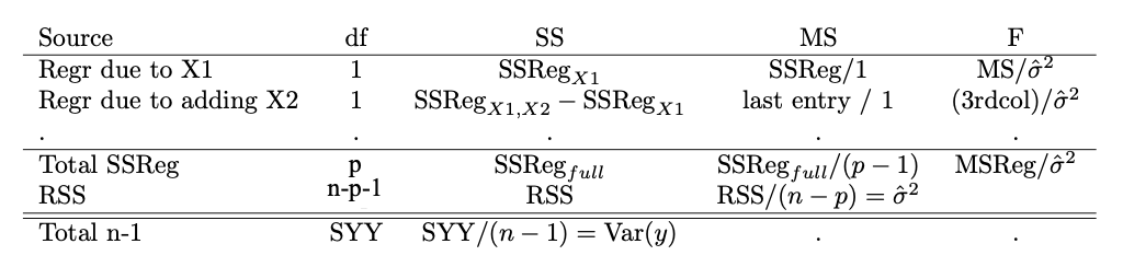
ANOVA table for partial test

sequential: individual contribution will be different based on what was explained by reduced model; assumes ONLY previous rows are included (not ones after!)

regardless of order, total SSreg will be the same

summary() and anova() often do not agree since summary() t.test output is not order based

they always agree when it’s the last variable added

adjusted r²

r² increases for any added variable, but adjr² accounts for additional predictors and whether or not they truly help

goes up when a new variable is useful, variable is otherwise insignificant

Variance Inflation Factor

measures collinearity, when predictors are linear combos of each other or measure similar info (height, weight)

having collinear predictors inflates their p-values

AIC

good model has small AIC

=reward for good fit + penalty for complexity

BIC

good model has small BIC

favors simpler models than AIC (though too low complexity induces bias)

=reward for good fit + penalty for complexity

Best subsets

set full model, decrease predictors by one; determine best by r²

use adjr², AIC, BIC, etc to judge which out of all sizes is best

Forwards/backwards stepwise regression

fwd: Fit size 1 model, keep best r²; fit all new models with two predictors, etc

backward: Fit full model; fit all new models with k-1 predictors and keep best, etc

Inverse response plot

transform of Y^lambda where lambda=0 is log transform

transforms WILL change interpretation, but ideally improve validity

BoxCox

transform of Y^lambda and/or predictors where lambda=0 is log transform, maximum likelihood estimation

gives a confidence interval

likelihood ratio tests, null is lambda=0 or lambda=1; if p is small, reject (do NOT do these transforms)

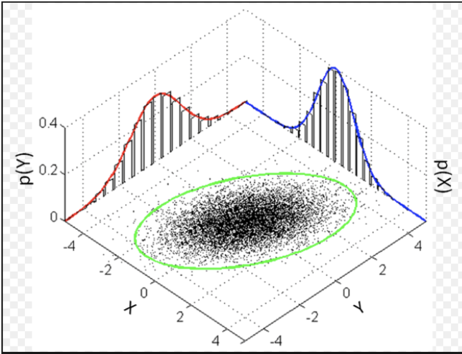
multivariate normal distribution

looks normal in 2d when you have nice ellipses

fitting different intercept and slope (categorical variables)

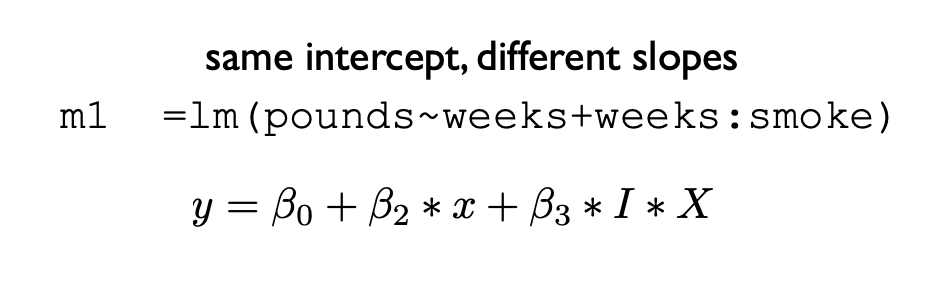
different slope: connect terms with :

different intercept: add terms with +