Lec 3 Topics in demand theory

P. Ushchev ULB, Solvay Brussels School of Economics and Management

own price elasticity of good i

ij-th cross price elasticity

income elasticity of demand for good i

the law of demand for good i holds if

ei > 0

the demand for good i is elastic iff

Ei > 1

otherwise it is inelastic

good i is a gross substitute to good j iff

eij > 0

otherwise gross complement

good i is normal iff

ni > 0

otherwise good i if inferior

the demand for goor i is income elastic iff

ni > 1,

otherwise it is income inelastic

why elasticities (instead of marginal effects)

elasticities are invariant to units of measurement (either physical or monetary): the values of derivatives will change if we switch from USK to EUR or from kg to pounds, while the values of elasticities will remain the smae

there are meaningful relationships between elastciities and budget shares

elasticities and budget shares

the budget share si(p,y) of good i

• decreases with pi iff the demand for good i is elastic

• increases in y iff the demand for good i is income-elastic

• increases with pj, i=! j, iff good i is a gross substitute to good j

what happens with the budget shares when the preferences are homothetic (similar)

the budget shares may depend on prices, but are independent of income

what happens when the preferences are indirectly additive → are representable by an indirect utility function of the form

then the budget shares have the logit-structure

Engel aggregation property + implications

there is at least one normal good (ni > 0)

when preferences are non-homothetic (non equal), there is at least one income-elastic good and at least one income-inelastic good

Cournot aggregation property + implications

when the demand for good j is elastic (inelastic), at least one good i≠j is a gross substitute (gross complement) to j

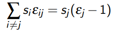
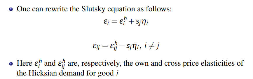
slutsky equation

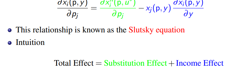
slutsky equation in the elasticity form

warning ; the elasticity matrix of the Hicksian demands need not be symmetric and negative semidefinite

basic idea of revealed preferences

consumer’s choices are viewed as revealed preferred to all other choices feasible under the same circumstances

Weak Axiom of revealed preference WARP → when does a dataset satisfly WARP

if the following consitions cannot hold simulatneaously

assume that we have some demand system x(p,,y) which satisfies budget balancedness and WARP, can this demand system be rationalized by a monotonic, strictly convex, and continuous rational preference over Rⁿ+ ?

for n= 2, the answer is positive, but negetaive for n>= 3

→ under n>= 3, revealed preference relationship may be non-transitive (WARP does not enforce transitivity across multiple intermediate steps)

→ therefore the Slutsky matrix of x(p,y) will be negative semidefinite, but generally fails to satify symmetry

How to cure non-rationalizability of WARP for n >= 3

Strong axiom of revealed preference (SARP), which os WARP + np intransitive cycle are possible

when is a demand system x(p,y) rationalizable ?

if and only if it satisfies SARP and budget balancedness

generalized axiom of revealed preferences GARP

is a counterpart of SARP for a finite dataset

how to deal with uncertainty ? the basic setting

Assume that

• there is a finite set of deteministic outcomes A = {a1,,,,,an}

• a consuùer has a preference over A: a1 >= a2 … >= an

assume that consumers may face not only deterministic, but also stochastic ooutcomes, → probability distributions over A

simple gambles

consider a set G of gambles over A

A simple gamble is a lottery which asigns porbabilities pi to outcomes ai

Formally, the set G’s of simple gambles is given by

Compound gambles

= lotteries in which “lottery teicket may be a prize”

in reasonable cases : when deterministic outcomes appear after finitely many steps, we still can compute the effective probability distribution of a compound gample : pi = P{a=ai}

axioms of choice under uncertainty

assume that a consumer has a rational preference >= over the set G of gambles over A, which satisfies the following requirements:

A1 A2A3A4→ see image

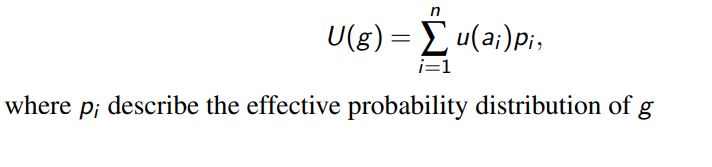
call a utility function U: G → R a Von Neumann Morgenstern utility iff : (VNM utility)

it can be represented as follows (image)

expected utility theorem

assume that rational preference >= over G satisfies A1-A4

then there exists a VNMutility representing >=

moreover, the coeff u(a1)..u(an) are uniquely defined up to a positive affine transformation, which means the following : (image)

what does the expected utility theorem mean ?

in the ocntext of the classical demand theoru, questions like “please grade yoru well-being using the 10-grade system” make no sense

such questions do make sense under uncertainty, given that we believe individuals truly compute expected utilities

indeed, if we choose the values of k and b so that u(a1)= 0 and u(an)= 10, then the 10-grade scale becomes a meaningful estimator of the expected utility level

risk averse

iff u(E(g)) > U(g) for any g e G0

and if the Bernouilli function u() is strictly concave over R+

wc (g) < E(g) for any g ∈ G0

P(g) > 0 for any g ∈ G0

risk neutral

iff u(E(g)) = U(g) for any g e G0

and Bernouilli function u() is affine over R+,

iff wc (g) = E(g) for any g ∈ G0

iff P(g) = 0 for any g ∈ G0

risk loving

iff u(E(g)) < U(g) for any g e G0

and Bernouilli function u() is strictly convex over R+,

iff wc (g) > E(g) for any g ∈ G0

iff P(g) < 0 for any g ∈ G0

certainty equivalent

Wc(g) is a solution to u(w) = U(g)

someone wants to buy your lottery ticket, whcih price woudl you accept

the risk premium P(g) of a monetary gable is a solution to

u(E(g) - P) = U(g)

→ P = E(g) - Wc(g)

why can the second derivative u’’(w) of the Bernouilli function (which captures concavity/convexity) not really be used to make comparisons of individual behavior ?

the numerical value of u’’(w) conveys zero meaningful information about individual behavior

how do we compare individuals regarding risk ?

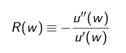
Arrow_Pratt absolute risk aversion

Consider two individuals, A and B, whose Arrow-Pratt risk aversion functions are, respectively, RA(·) and RB (·)

Assume that A is more risk-averse than B in the following sense: RA(w) > RB(w) for any w ≥ 0

Then, for any non-degenerate gamble g, A’s certainty equivalent is lower than B’s: w ^A c (g) < w ^B c (g) for any g ∈ G0

image

DARA

decreasing absolute risk aversion