psy201 lecture 1

lecture 1

Data source: population parameter

come from the entire population of interest

• data in pop

Data source: Sample statistics

subset taken from the population, usually when access to the population is not possible. These are usually generalized to the population

• data in sample

Statistical calculation: Inferential statistics

used to generalize information or make predictions

• how we infer

Statistical calculation: Descriptive statistics

Denote information about the set of data, such as the mean and standard deviation

• how we describe data

Expected values

What is predicted to occur. “We expected a value of 100”

Observed values

are what we actually measure. “We observed a value of 120”

how to ensure good validity

done through proper experiment design, like random selection and random assignment

External validity

is how well the data represents the population of interest

Internal validity

is how well the data measures the construct of interest

Reliability

how likely that numerous measurements will report similar observations to previous ones. Validity and reliability can be contrasted

Categorical data vs measurement data

Categorical data have discrete boundaries

Measurement data are continuous in nature

Nominal data

includes categories with no hierarchical relationship (i.e., all categories are weighed equally)

• Nominal data have no hierarchy or numeric value between them

Ordinal data

are categorical variables but there are hierarchical relationships

• Ordinal data have hierarchies but these are not numeric, in other words the hierarchy is not additive

Interval data

are measurements with equal distances, but no true zero. They have additive relationships

• Interval data measurements are hierarchical based on an additive values, but are not multiplicative

Ratio data

is measurement data with equal distances, and a true zero. Thus there are additive and multiplicative relationships

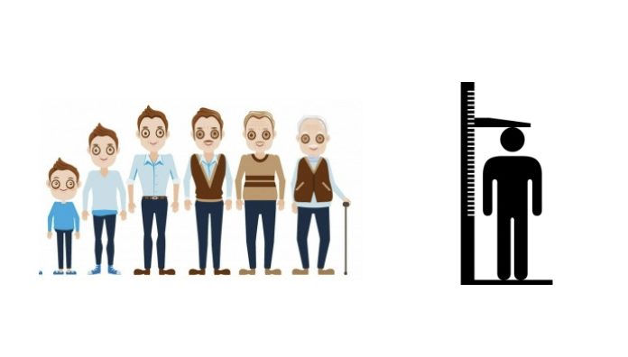
convert between categorical and measurement data

third variable

one that is related to the dependent variable, which can also explain the observed effects

confound

alternative explanation where there is some unique manipulation alongside the

dependent variable that is not accounted for. Think of “drug” and “no drug” conditions

Efficiency

how much data do we need for a variable to be a good estimate

Sufficiency

how much data is used to create an estimate

Bias

whether the variable is likely to overestimate or underestimate the true value it is estimating

Resistance

how much influence do deviant scores like outliers have on the estimate

truncate

We can truncate the figure, where the Y-axis does not start at zero, which

magnifies hard-to-see differences. Though interpret this with caution

because it can be misleading. Politicians love this nasty trick!

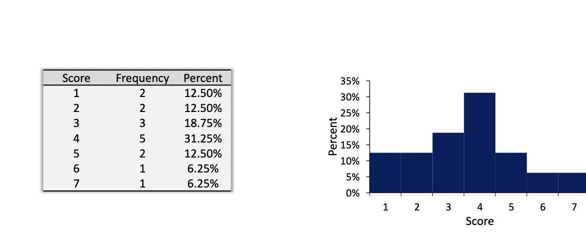
relative frequency histogram

shows the percent of each score of the total rather

than the raw numbers. This can be easier to understand the quantity of scores

relative to the entire dataset. Captured by dividing the frequency over N

cumulative frequency histogram

each bar includes the sum of the previous

values. This shows a total increment. It is good for data where not many changes

occur at each interval, or you want to display an aggregate

• As an example, displaying research publications over time

Binning

Method to combine intervals into smaller

increments. This is useful when your variable has a wide range

Descriptive data

summarizes data into few, representative values. For example, listing

out the individual ages of students in a class is not informative. And a figure, while

useful, is not a summary

Central tendency and Measurement of spread

Central tendency provides a single value that is representative of the overall data

Measurement of spread describes how scores typically vary from the central tendency

mean is the least squared distance

considered the “true average, It takes all scores into consideration equally, and it is the closest point to all score equally.

Interquartile range (IQR)

is the range of the middle 50% of the data. This involves calculating

three sets of medians. Once again, the data needs to be rank ordered

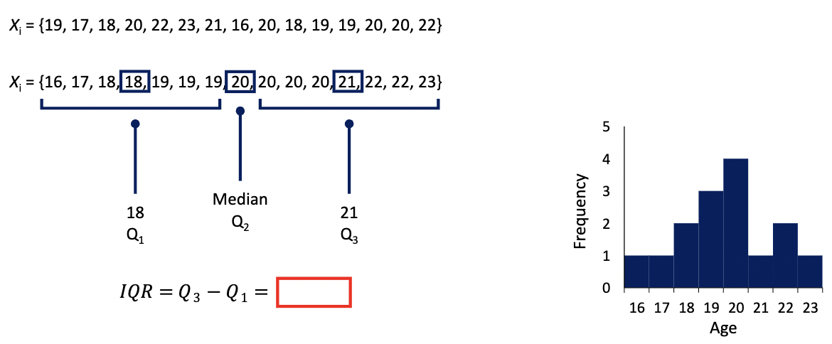
IQR use over range

The IQR can be more useful than the range when there are many highly deviant scores. For example,

when looking at final grades, there will be students who receive very low scores (single digits) and

others who receive 100s. But the “bulk” of scores will be in the 60-70s range

IQR is typically plotted in a box and whisker plot

variance

the average squared distance scores are from the mean

two parts of variance

the sum of squared differences (SS), and the denominator to average (N, or df)

• Differences are squared, else the sums after subtracting from the mean will be zero

degrees of freedom (df). (n-1)

This is a modification to the denominator to

account for the fact that sample variance (and sample standard deviation) is not an unbiased estimator

of the population variance or population standard deviation. We will talk about this next lecture. Sample

mean is an unbiased estimator of the population, and so it does not need a correction