1042 FINAL EXAM BIOSTAT

How does Biostatistics and Epidemiology go hand in hand?

• For a good data analysis, you need good data

• Epidemiologists involved in study design & data collection

What are some features of Normal Distributions (7)?

• Normal distributions are symmetric around their mean

• The mean, median, and mode of a normal distribution are equal

• The area under the normal curve is equal to 1.0

  • Because the area under the curve is the cumulative sum of relative frequencies (which has to be out of 1)

• Normal distributions are denser in the centre and less dense in the tails

• Normal distributions are defined by two parameters, the mean (μ) and the standard deviation (σ)

• 68% of the area of a normal distribution is within one standard deviation of the mean

• Approximately 95% of the area of a normal distribution is within two standard deviations of the mean

Example: The BMI for the adult Australians follows the normal distribution with mean 28 kg/m² and standard deviation of 2 kg/m². We want to calculate the probability that a randomly selected person from this population has a BMI greater than 25 kg/m²

1. Calculate the Z-score = – 1.50

• Z-score = (Observed Value – True Mean)/(True Standard Deviation) = (25–28)/2.0 = −1.5

2. Open the normal probability table

3. Consider the absolute value (always positive) of the Z-score and break it into two parts:
   (a) the whole number and the tenth and
   (b) the hundredth
   In this example, the absolute value of the Z-score is 1.50.
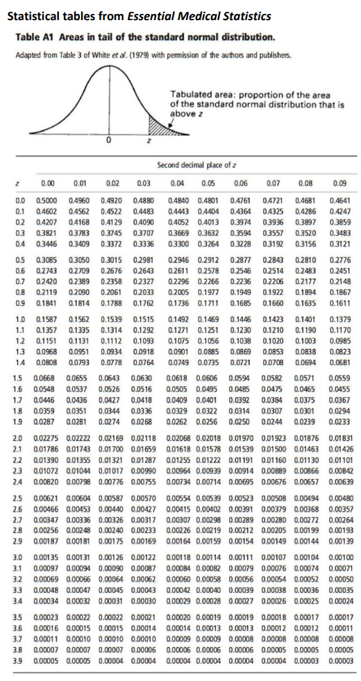
   The whole number and the tenth is 1.5 and the hundredth is 0.00

4. The whole number and the tenth (1.5) are looked up along the first column and the hundredth (0.00) is looked up across the first row in the table

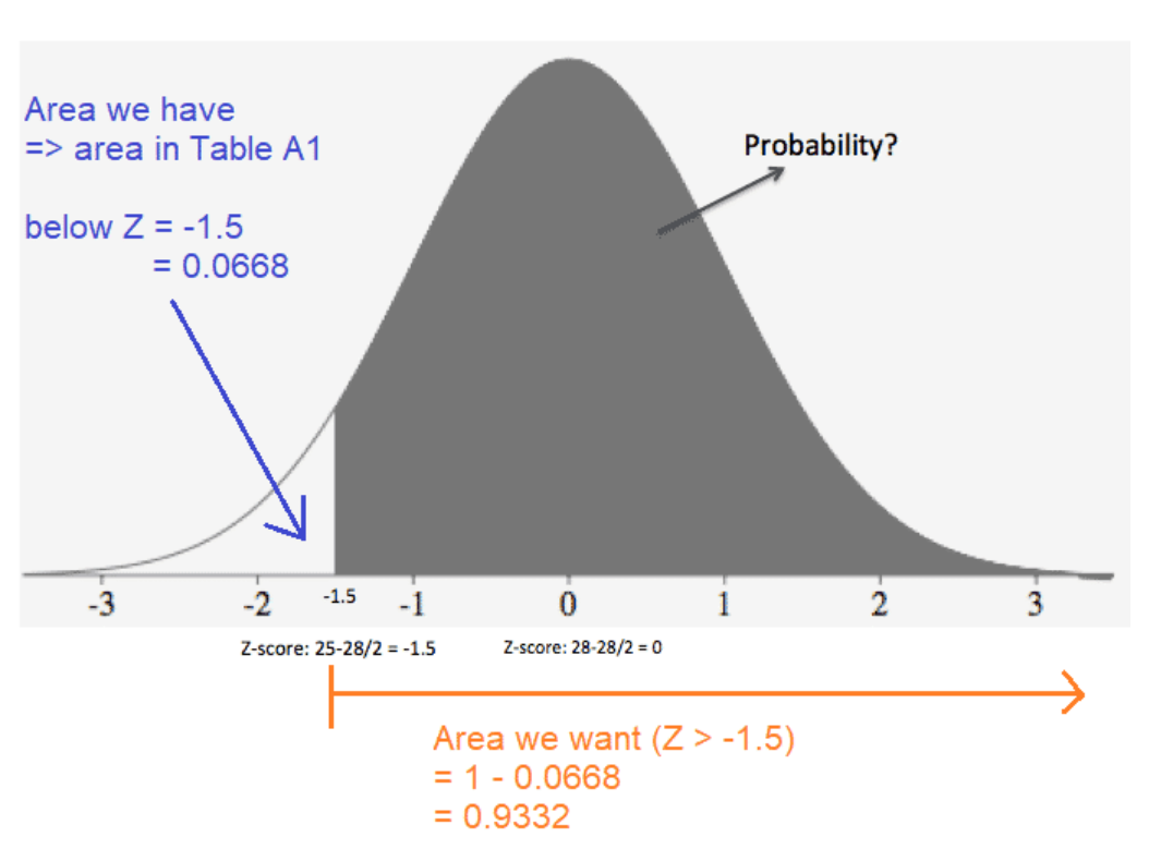
5. The value in the intersection of the row and column is the probability from the absolute value of the Z-score to infinity (i.e. above the Z score). Thus from the table, the probability above 1.5 is 0.0668
   Note: Due to the symmetry of the normal distribution, the probability below -1.5 is the same as the probability as above +1.5.

7. We are interested in the probability of a Z-score greater than -1.5.
   The easiest way to calculate this is: 1 - 0.0668    (i.e. entire area - [area below -1.5]).

8. Thus the required probability is 0.9332  (1 - 0.0668)
   
   Hence the probability that a randomly selected adult Australian is overweight (BMI > 25 kg/m²) is 93.32 %

How to use the row and column in the z-score table

• Row = whole number + first decimal

  • For example, if your Z‑score is 1.50, you go to the row labelled 1.5

• Column = second decimal (hundredth place)

  • The top row shows 0.00 to 0.09.

  • If your Z‑score is 1.53, you move to the column labelled 0.03

E.g. So, for Z = 1.50, you use row 1.5 and column 0.00, giving 0.0668. If your Z‑score were 1.56, you’d use row 1.5 and column 0.06, giving 0.0606.

How to do Normal Distribution calculations on Excel?

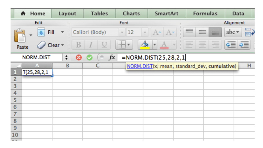
• “=NORM.DIST”

• The NORM.DIST function calculates the probability the variable X falls below a specified value

• =NORM.DIST(x,mean,standard_dev,cumulative)

  • X is the observation point (what you want)

  • mean is the true mean

  • standard_dev is the true standard deviation

  • cumulative is whether you want a discrete or cumulative probability

  For the above example: =NORM.DIST (25, 28, 2, TRUE) =0.0668 ⇒  1 – 0.0668 = 0.9332 or 93.32%

What is a Parameter?

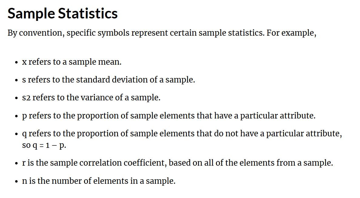
• A parameter is an unknown characteristic of interest in the true population

• Parameter describes an entire population is denoted by Greek letters

• General examples include the true mean, true proportion, and true standard deviation

• It is difficult to calculate for a large population due to financial and time constraint

  • An example: Consider the BMI of Australians of age 30 to 60 years. If all the Australians within this age groups are taken into account to calculate the mean and standard deviation of BMI, they are called the true (population) mean and standard deviation respectively

    If we calculate the proportion of patients within the population who are obese (BMI > 30 kg/m²), the proportion is called the true (population) proportion

What is a Sample Result?

• The estimated value of the parameter based on a random sample taken from the study population

• Statistics describe a sample and are denoted by Latin (roman) letters

• General examples include the mean and proportion in the sample

• The calculated values for the sample data are used to estimate parameters

• If we take a random sample from a population and calculate the mean for this sample, then this mean is known as the sample estimate of the population mean or simply the sample mean

Box plot outliers example

Lower outlier threshold = Q1 -1.5 x IQR = 7.3

Upper outlier threshold = Q3 + 1.5 x IQR = 19.3

• Therefore, when you draw your min and max you need to use the min and max given so long as they are not outside the upper/lower threshold, if your min was 1, then on the box plot you whisker ends at 7.3 and the data point 1 will be a point outside the whisker

Risk Calc

Relative risk → Higher risk/Lower risk

Absolute Risk → %

What is the correct classification of data so important?

• Because it determines the types of graphs that need to be used, the type of summary statistics as well as the statistical analysis needed

• SUMMARY STATISTICS INCLUDES MEAN, MEDIAN, MODE, SD, RANGE

How to categorise Data

• Categorical

  • Nominal (order of categories doesn’t matter) e.g. Blood group (A, B, O, AB) e.g. Diabetic (Yes / No) Also known as “binary”

  • Ordinal (order of categories does matter) e.g. BMI (underweight, normal, overweight, obese) e.g. Pain severity (None, Mild, Moderate, Severe)

• Numerical

  • Discrete (counts) e.g. Number of hospital admissions

  • Continuous (measurements) e.g. Weight, Height, BMI, blood pressure, cholesterol, etc

Data transformation

• ONLY ONE WAY Continuous → Categorical

• So we have out continuous BMI data that we get from calculating Weight (Kg)/Height²

• And then we can use that continuous data to put make categories such as weather the person is underweight, healthy weight etc.

• We cannot use categories and then make up continuous data

Population Vs Sample?

• The population: The entire collection of patients of interest, as defined in the study design

  • E.g. All diabetics in Australia

• Actual population of interest often large

  • Can’t measure everyone – expense, time, etc

  • Exception = Census (every 5 years)! (2011, 2016, 2021, etc)

• Solution: Take a sample that is representative of part of the population of interest. Collect data for this sample.

  • E.g. Sample of 100 diabetics in Australia

  • Use this data to make inferences about the population of interest

  • Don’t forget: Behind statistics & studies are people!

Sampling Level

• Sampling is normally at the individual level

• Other times (when investigating an intervention), it is at a “cluster” level

  • House, School classrooms, or schools, Hospital wards, or hospitals

Types of Sampling Methods

• Simple: Sampling frame is everyone doing BMS1042. Numbered 1 to 700. Randomly select 10 numbers → Those students are selected

  • Everyone has the same chance of being selected, can be expensive

• Stratified sample: Have list of everyone in each biostats tutorial. Randomly select 5 students from each tutorial using “simple” method above

  • Can be unbiased and representative, but time consuming

• Cluster: Tutorial rooms have 15 tables with 6 students on each. Select 2 tables

  • More coinvent that simple, but could be bias

• Systematic: Select every 20th student on the roll, starting with 15th

• Convenience: Tutor picks a couple of groups of 6 students in the tutorial room. (Both are near where the tutor is standing at the time) save times

  • Usually biased, could pose self-selection bias where people want to participate because they know more about this topic

• Snowball sampling: Criteria = wear glasses

  • Start at the nearest table – find a student who wears glasses. Stand up. Then they find others wearing glasses = stand up too, therefore selected

  • Quite liable to bias, people tend to associate with people with similar characteristics hence harder to apply results to the wider population + researcher needs to be kind to the participant doing the referrals

*Note the probability vs non-probability types of sampling

*There will ALWAYS be sampling error since we cannot copy paste a population exactly

*When you have 2/3 red people and 1/3 blue people in the population, then there should be the same ratio in the sample

When to use each sampling technique

• Simple Sampling → Used when the target group is sufficiently large. Do not use SRS when the target study group is a relatively small subgroup that might be missed by this method.

• Stratified → Used when there are smaller sub-groups that are to be investigated, you want to achieve greater statistical significance in a smaller sample and use it to reduce standard error

• Systematic → Used when it is difficult to identify items using a SRS method (with random numbers). Used when it is easier to select every nth item (instead of making a whole ass list and numbering it as with SRS)

• Cluster → Used when the studied population is spread across a wide area such that SRS would be difficult to implement in accessing the selected sample

• Snowball → Used when you do not have access to sufficient people with the characteristics you are seeking

Snowball sampling example

• Find people who meet your criteria. Ask them to refer you to others.

  • E.g. The Burnet Institute recruit people for many studies where there is no “list” of eligible people. For example. Injecting Drug Users (IDU)

• Think about how viral social media posts work amongst your friends

• Person 1 sees an awesome post on their News Feed, and hits “share”. Some of their Friends see it, and “share” it, etc.

• Sampling people via snow ball sampling is like social media “share”.

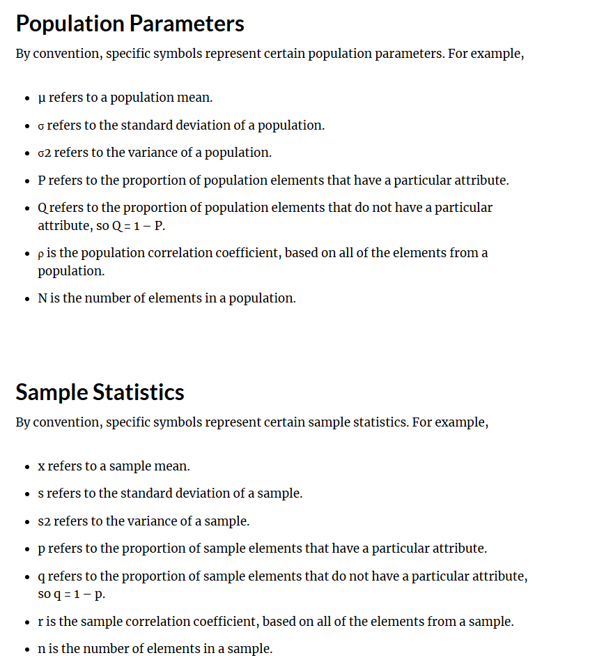
Notation

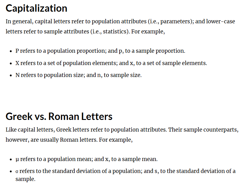
• Capital letters → Population (P), lower case letter → refers to sample (p)

  • N refers to population size, n refers to sample size

• Greek Letters → population attributes, normal letters → sample attributes

  • μ refers to a population mean; and x, to a sample mean

Big picture or Biostatistics

1. Note population, develop topic

2. Data collection (via sample)

3. Data Analysis

4. Making an inference with the data collect from the sample onto the wider population

*The two basic divisions of statistics are inferential and descriptive

How can data be organised?

Observations

• Information from a patient or experiment is called an observation

• An observation may represent single or multiple pieces of information about a patient

• Examples include: age, gender, height, weight, blood pressure level and cholesterol level of a single patient

Variables

• A variable is any observation that can have different values

• A variable may have different values when observed at different times for the same patient.

• A variable may have different values for different patients.

• If we consider the blood pressure of patients in a study, it is likely that the blood pressure for each patient will be different, thus blood pressure is a variable.

Population vs Sample definition

Population

• A population is the largest collection of entities for which we have an interest at a particular time.

• The term target population is often used in scientific literature to define the population of interest.

• Example: the incidence of ovarian cancer of women between the ages 25 to 55 years in Australia → the population in the example is all women in this age group in Australia.

Sample 

• Defined simply as a representative part of a population and consists of one or more observations from this population.

• The sample is a section of the population that represents the population as much as possible.

• Consider the diabetic population in Victoria. If we collect fasting blood glucose levels of only a fraction of these patients (e.g. 5 patients), we have only a part of our population and thus we have a sample.

What are different ways to present categorical data?

Relative Frequency

• Relative frequency = % in each category

  • Can be presented in a table/ graph

• Tabulate the number of observations in each category

Crosstab

• Tabulation of the number of observation - in each combination of categories (e.g. Disease and Pesticide exposure)

  • Can then be used to calculate row% (%developed disease, by pesticide exposure), or column% (%exposed to pesticides, by disease status)

Expanded Table

• Many different summaries

• Attack rate (% of those who ate the food that got ill)

• Relative risk (Risk exposed/ Risk unexposed)

Cross Tabulation of 2 categorical variables

Which % (row or column) better? It depends on your question

• Overall, 22.80 % (145 / 636) had respiratory symptoms

• 77.20 % (491 / 636) had no respiratory symptoms

• 24.18% (81 / 335) of females had respiratory symptoms

• 21.26% (64 / 301) of males had respiratory symptoms

• Overall, 52.67% (335 / 636) were female

• 47.33% (301 / 636) were male

• 55.86 % of those with respiratory symptoms were female

• 51.73% of those without respiratory symptoms were female

• Which overall % makes more sense?

  • Respiratory symptoms

  • Therefore row % best in this case

*Always work out OVERALL, and then go into the table and see what you need

Row% and Column%

• Depending on the situation:

  • Sometimes the row % is appropriate.

    • The row % represents the outcome that can then be separated into various patient characteristics categories (e.g. Developed influenza %  in "received vaccine" and "received placebo" subgroups)

  • Other times the column %is appropriate.

    • The column % represents the patient characteristics that can then be separated into various outcomes. This is often used in a Table 1: Patient characteristics in a paper. (e.g. Received the vaccine %   in "developed influenza" and "did not develop influenza" outcomes)

  If unsure, calculate and interpret both. Often writing out what the % represents in words will help you work out which % is best for the situation you're considering.

Descriptive statistics for Numerical continuous data

Central Tendency

• Mean (Average = sum of observation/ no. of observation)

  • Suitable when data is normal and not skewed

• Median (middle value) - good for skewed data/outliers

• Mode (most frequent measurement or [range'] - in a histogram)

Variation

• Standard deviation - variation in observation from mean

• Interquartile range [IQR] = 3rd quartile minus the 1st quartile

Central Tendency Measures

Mean= Sum of all values / no. of value

• Excel: AVERAGE(A1:A2)

Median

• Not affected by extreme values - hence commonly used in asymmetrical data

• Excel: QUARTILE(A1:A2,2) OR Excel is =QUARTILE.INC(range,2)

Mode

• A distribution with one mode is known as uni-modal, with two modes is bimodal and similarly having more than two modes is called multi-modal

• The mode is can be useful for categorical data and numerical data

• Excel: MODE(A1:A2)

Symmetrical Data

• For symmetric data the mean, median, mode are approximately the same

• If we are comparing summary statistics (averages) for multiple groups of patients where all groups are symmetrical, the mean should be reported for each group

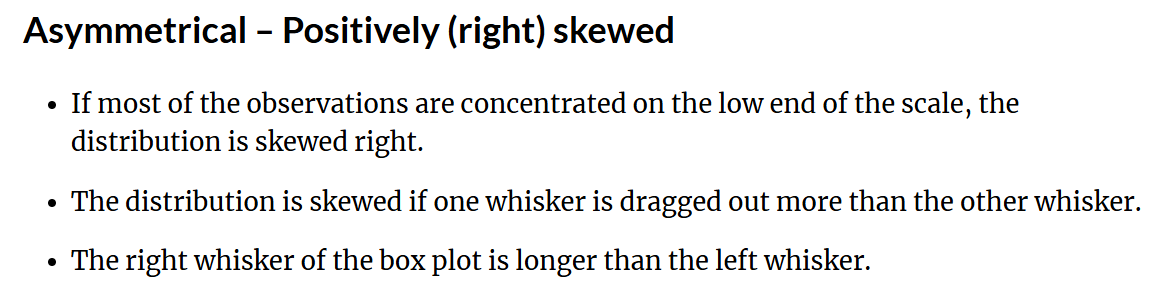
Positively (right) Skewed (Asymmetrical data)

• For positive skewed data the mean ≥ median ≥ mode

• If we are comparing summary statistics (averages) for multiple groups of patients where one or more groups is/are positively skewed, the median should be reported for each group

• For example: Postoperative length of hospital stay (LOS) of cardiac surgery patients presented in figure below is positively skewed. Hence the mean LOS is higher than the median LOS and median LOS is higher than the mode LOS

Negatively (left) Skewed data (asymmertircal data)

• For negative skewed data the mean ≤ median ≤ mode

• If we are comparing summary statistics (averages) for multiple groups of patients where one or more groups is/are negatively skewed, the median should be reported for each group

• For example: Age of cardiac surgery patients presented in figure below is negatively skewed. Hence patients mean age is lower than median age and median age is lower than modal age

What are the different types of graphs?

• Bar chart

• Pie chart

• Scatterplot

• Histogram

• Box plot

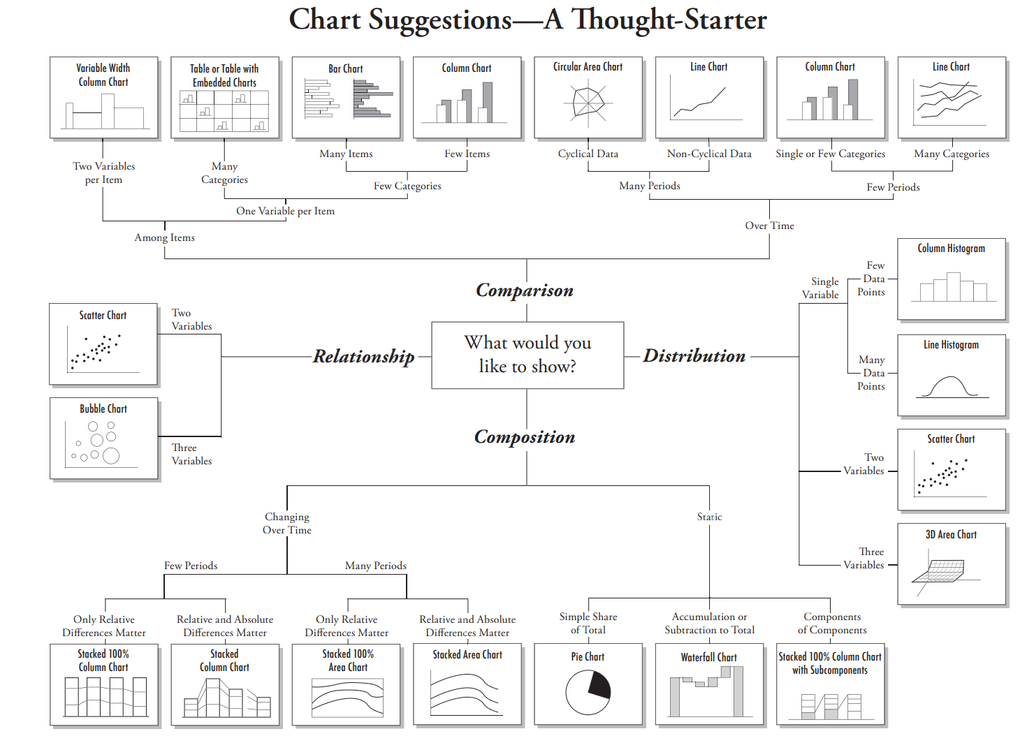
Graphs are good for comparisons, identifying relationships, describing distributions and visualising compositions. See the document below for further information.

*Graphs tells a story and need to stand alone

Tables are a way of summarising “raw” data (categorical = frequencies, Numerical = summary statistics)

Bar Chart

• Bar charts are used to: 

  • Summarise the data

  • Illustrate categorical, composition and comparative data

  • Present visual representation of data that might otherwise be provided in a frequency table.

  What you need: 

  • Each category to be independent of one another (mutually exclusive)

  • Categorical data of both nominal or ordinal nature

  • Discrete (but not continuous) data sets can be used for bar charts

• Should be standalone, so you can infer the information from the axis and title, without the need of accompanying text

• A bar chart is superior to pie charts due to larger amounts of categories that can be utilised

• TO create a bar chart you need to: calculate the relative frequencies

How to interpret a bar chart

• Percentages for each category in descending order

• The largest (and second largest) percentages and why these are significant

• The smallest percentage and why this is significant

• Summary conclusion – bringing it all together

Pie chart

• Pie charts are used to: 

  • Summarise the data

  • Illustrate categorical, composition data

  • Present visual representation of data that might otherwise be provided in a small table (clarify trends better than frequency tables)

• What you need: 

  • Each category to be independent of one another (mutually exclusive)

  • Categorical data of both nominal or ordinal nature

  • Fewer than 6 categories ( ≥ 6 categories in a single pie chart can be difficult to interpret )

• Fails to reveal key assumptions, causes, effects or patterns

• Have to add up to 100% - REPRESENTS RELATIVE FREQUENCY (summary statistics)

• Categorical data - can only graph one variable at a time

How to interpret Pie charts

• Percentages (%) for each category in descending order

• The largest (and second largest) percentages and why these are significant

• The smallest percentages and why this is significant

• Summary conclusion – bringing it all together

Scatterplot

• Scatterplots are used to: 

  • Summarise the data.

  • Show a relationship between two sets of data AND Display the distribution of data

• What you need: 

  • Two quantitative variables x and y.

  • X variable may be numerical or categorical, the Y variable must be continuous.

  • Graph to plot your data with an x (horizontal) and y (vertical) axis.

• Each dot represents one data point

• Can sometimes sure a line of best fit

• Assumptions: Observations in our data set are independent 

• Numerical, continuous data for BOTH axis

How to interpret scatter plots?

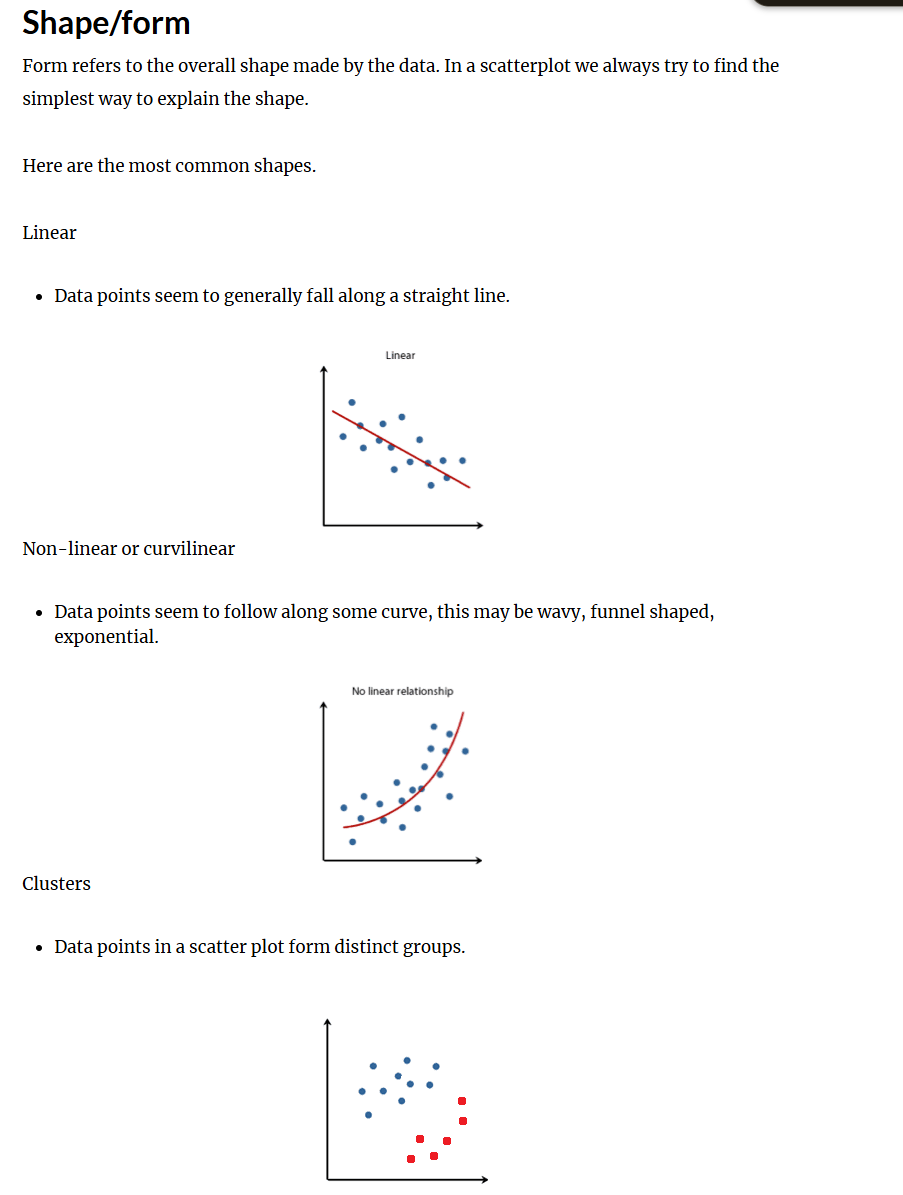
Overall Pattern

• Direction - positive, negative neither (above)

• Shape - Liner, non-liner, clusters (below)

• Strength - Strong relationship, Weak relationship (google this)

Deviations from pattern

• Outliers

Histogram

• Histograms are used to: 

  • Summarise the data

  • Illustrate numerical data

  • Help visualise and interpret the distribution of a data set

• What you need: 

  • Numerical data that is only continuous in nature.

  • Each observation or data point is independent to one another

• Bars touch

• Blocks are proportional in area to the frequency in each class

• Represent COUNTINOUS data, but are displayed like a bar chart

• Histograms display the distribution of a data set, whereas bar charts are used to compare variables

How do we figure out the width of the intervals for histograms?

• You don’t need to start from zero

Boxplot + quartiles

Q1 = 1st quartile, median of the lower half of the data (25th percentile - 25% of data is below that value) INCLUDE THE MEDIAN

Q2 = 2nd quartile = Median

Q3 = 3rd quartile, median of the upper half of the data (75th percentile - 75% of data is below that value) INCLUDE THE MEDIAN

• Dots represents outliers = outside 1.5 box-lengths from Q1 or Q3

  • Extreme value = outside 3 box-lengths from Q1 or Q3

• Graphs numerical data (discrete and continuous)

• Lower and upper whiskers = vertical lines

  • Length of lower whisker = Q1 – 1.5 x IQR

  • Length of upper whisker = Q3 + 1.5 x IQR

Inter-quartile range (IQR)

Inter-quartile Range (IQR) = Third Quartile ( Q3 ) - First Quartile ( Q1 )

• The advantage of the IQR is that it calculates the spread among the middle 50% of the observations only and thus is not affected by the extreme values. Like median, the IQR is commonly used for comparing asymmetric data

• Excel: subtracting Q3 [=QUARTILE.INC(range,3)] and Q1 [=QUARTILE.INC(range,1)].

When are box plots used?

• Present the distribution of numerical data (discrete and continuous)

• Compare two different data sets (comparison) in parallel box plots

• Identify outliers and comparing distributions for multiples groups

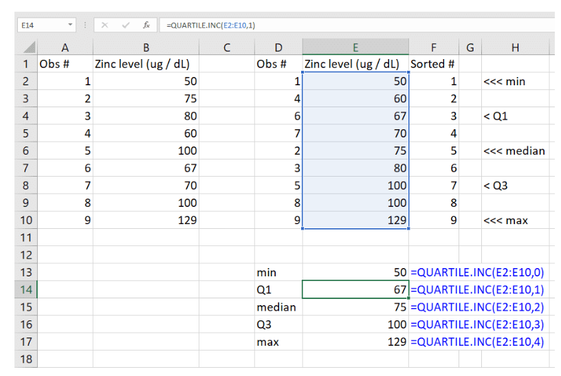
How to calc quartiles on excel?

QUARTILE.INC(array,quartile)      
This includes the minimum & maximum values when calculating quartiles

• array = is the range of cells that you want to calculate the quartile for (e.g. A1:A2)

• quartile represents the quartile being calculated
  0 (min) ; 1 (Q1) ; 2 (median) ; 3 (Q3) or 4 (max)
  
  

How to calculate SD?

• This is the most widely used measure of variability for symmetric data and is the average distance of the observations in the data set from their mean

• When the values of a set of observations lie close to their mean, the standard deviation is less than that when they are scattered over a wide range

• Excel: =STDEV.S(range)

Distribution of Data

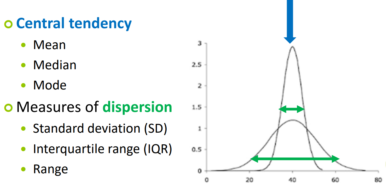
• Look at the tail

• Normal distribution = nominally distributed

• Distribution has two parameters:

  • Central value => Mean (Mu,µ)

  • Spread => Standard Deviation (Sigma,σ)

What is the aim of descriptive biostats?

Aim

• Identify health objectives i.e. National Health Priority Areas

• To assess the health status of a population i.e. Millennium Development Goals

• Allows allocation of resources efficiently by targeting populations

Frequency Tables

Frequency Table & Relative frequency example

• Gender is NOT BINARY - it is categorical, nominal

If the data is:

• Symmetric (normal) you will be reporting the mean and SD

• Asymmetric (skewed) you will be reporting the median and SD

What are some population parameters and Sample Statistics?

=STDEV() in Excel

What are some commonly used distributions?

• Bernoulli distribution (rarely used/not covered in this course)

  • Only for samples of size 1!

• Binomial distribution

  • Two mutually exclusive events

  • Probability of interest (pi) known

  • The number of times an outcome repeats in a data set

• Normal distribution

• T – distribution

• Chi-square distribution

What are the Reference ranges for the Normal Distribution?

• Normal distribution is also known as the Gaussian distribution

• Appropriate for continuous data

• Symmetric and bell shaped

• Distribution has two parameters: Central value => Mean (Mu,µ) AND Spread => Standard Deviation (Sigma,σ)

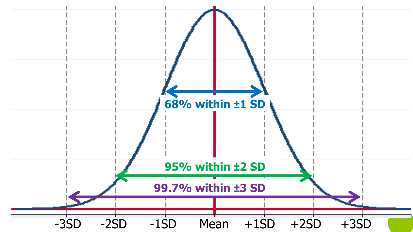
What is the 68 – 95 – 99.7% RULE?

If data follows the normal distribution:

• 68% of observations fall within the range (Mean – 1 SD) and (Mean + 1 SD)

  • The chance a random obs falls b/w - 1SD and +1 SD is 68%

• 95% obs fall b/w (Mean – 2SD) & (Mean + 2SD)

  • The chance a random obs falls b/w -2SD and +2 SD is 95 %

• 99.7% obs fall b/w (Mean – 3SD) & (Mean + 3SD)

  • The chance a random obs falls b/w -3SD and +3 SD is 99.7

REVIEW QUESTION FOR REFERENCE RANGES

a) Normal distributions where mean = median = 20

b) 68%

c) 10-30

---

What is the probability that a patient will have an ICP above 27.5 mmHg? → need to use Standard normal distribution since there is no +1/2 SD between them

What is the Standard Normal Distribution?

• Standardised Normal Distribution → with set parameters: Mean = 0, Standard Deviation = 1, Uses “Z-score” (this Z-score just says how many SD away from the mean is the observation)

• Used when reference range not suitable

• If the true mean & SD unknown, the sample mean (0) & SD (1) can be used when the sample size is large (30-40+)

• Intracranial pressure (ICP) example:

  • Mean = 20 mmHg, SD = 5 mmHg

  • Observed value = 27.5 mmHg

• Thus 27.5 mmHg is 1.5 SDs away from the mean

How to calculate using the z-score

Intracranial pressure (ICP) example:

• Mean = 20 mmHg, SD = 5 mmHg

• Observed value = 27.5 mmHg

• 
  

Finding the probability that the ICP > 27.5 mmHg

Step 1: Draw a diagram (above)

Step 2: Calculate the Z-score (Z = 1.5) using equation: Observed Value (27.5) - True Mean/ True SD

Step 3: Look up the value in Table A1 (Standard normal table)

Step 4: Work out the appropriate probability

• Probability (Z > 1.5) = 0.0668 (from Table A1)

• Thus the probability ICP is greater than 27.5 mmHg is 6.68%

What are some other scenarios for using the Standard Normal Distribution?

• ALWAYS draw a diagram first!!!

• Always note which part of the table is shaded, for example rn we have values on our table given z<, but some tables only give 0-z

What is “SAMPLING DISTRIBUTION”?

Step 1: Take repeated independent samples (n) (same size) from the true population (N). Calculate the mean BMI for each sample

Step 2: Record the sample means

Step 3: Present the results (sample means) on a Histogram. This histogram is called the “sampling distribution”

Step 4: Calculate the mean and standard error (which is the standard deviation of the means) from the sample means

If the population distribution is skewed then the sampling distribution of the sample mean will NOT be skewed → central limit theory

For a sufficiently large sample the sample means arising from repeated samples will cluster around the population mean

A sample mean from a larger sample is likely to lie closer to the population mean than a sample mean from a smaller sample

What is/are CORRECT regarding the mean of a sampling distribution?

• It is the mean of the statistic for all of the samples in the distribution

• It is the same as the population parameter

What is the Central Limit Theorem?

For a large sample size, the distribution of the sample mean is normally distributed, even when the population distribution from which the sample has been drawn is decidedly non-normal, with mean equal to the true mean of the sampled population and standard deviation equal to the standard error of the sample mean

• The same mean becomes more concentrated around the population mean in LARGE samples

• As SE decreases, the sample mean approached the population mean

• Small sample size - distribution of sample mean is more spread out

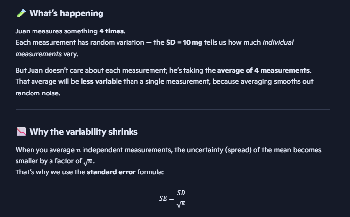
What is Standard Error (SE)?

• We do not use repeated sampling for calculation of standard error instead we draw a random sample from the population and calculate the sample standard deviation

• SE is the Standard Deviation of the distribution of the sample mean

• Measures the dispersion (spread) of the sampling distribution

• Measures how precise the population mean is estimated by the sample mean

• Technically: Standard Deviation of the distribution of the sample mean

*Does not increase as sample size increases :,)

SE question

How does sample size and SD change SE (per equation)

The 68 – 95 – 99.7% rule and Sampling Distribution

If the “mean” is the sample mean that is taken from a population …

• 68% of sample means are expected to lie between (µ – 1SE) and (µ + 1SE)

• 95% of sample means are expected to ‘lie between (µ - 2SE) and (µ + 2SE)

• 99.7% of sample means are expected to lie between (µ - 3SE) and (µ + 3SE)

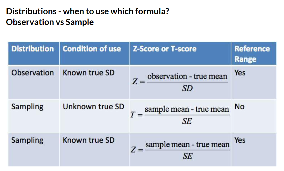
What is the T-score?

• We can’t always use the reference ranges for the sampling distribution

• So we use the Z-scores or T-scores instead

• T-score

  • Used when the Population (true) Standard Deviation is unknown, and we only have the Sample Standard Deviation

• Z-score

  • Used when the Population (true) Standard Deviation is known

How to calculate the Z-score with a standard error (SE)?

The birth weight in a hospital follows the normal distribution and the population mean and SD of birth weight are respectively 112oz and 20.6oz.

What is the probability that the mean birth-weight from a random sample of 100 infants from this hospital will be between 107.571 and 116.429 oz?

107.571 and 116.429 oz are sample means hence we

• Think of SD as the “noise” among individuals, and SE as the “noise” among averages

• Since SE measures variability among sample means if you repeatedly took samples of size 100 from that population the mean would fluctuate. Therefore by averaging over 100 babies smooths out random fluctuations, so the uncertainty in the mean is smaller — that’s what SE quantifies

Look at the A1 table:

• Area in the tail for z=2.15 => 0.01578

• Therefore the area we want is 1 - 0.01578 - 0.01578 = 0.96844

• The probability that the mean birth weight of a random SAMPLE of 100 infants will be between 107.571 an d116.429 oz is: 96.84%

How to calc T-Score with standard error (SE)?

Note for SE we are using the sample SD instead of the population SD

The T-distribution and its relationship to the normal?

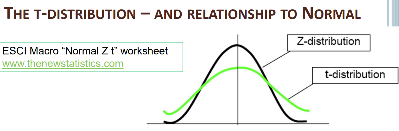
• Very similar to the normal distribution

• Symmetric & bell shaped

• Bell (peak of curve) is flatter than the Normal distribution

• Tails are longer than the Normal distribution

• df = Degrees of freedom. Number of observations that can change

• As the sample size (and df) increases, t → (gets closer to the) Normal

T-score, example

• Look up t = 1.38, df = 9 in the T-distribution table

• The one-sided tail T-distribution value = 0.10

• Thus the probability that in a random sample of 10 newborn babies, the sample mean will be above 121 oz is 10%

How to use the T-distribution table

Look up t = 1.38, df = 9 in the T-distribution table

• Find the df of 9, and then search for 1.38, then look up

• In this case we only want one tale, therefore we look at ‘one-sided P-value’ → 0.1

• Thus the probability that in a random sample of 10 newborn babies, the sample mean will be above 121 oz is 10%

---

• If the df is above 120, consider that the df = infinite (via looking at the table notes)

• Use a df in the table that is closest to the df value you need (e.g. a df=49, can be approximated by using the df=40 on the table

What are Degrees of Freedom?

• df = Number of pieces of information that was used to estimate another

  • E.g. Total DBP of 4 students = 280 mmHg

  • Therefore when we ask for 4 obs, initially the obs did not add up to the total

  • Therefore the 4th obs had to be 70 not 50

  • Therefore obs1,2,3 could be chosen (df = choose)

  • But obs 4 had to be fixed

  • Hence df = 4 -1 =3, because we have 3 degrees of freedom in this example

• The higher the df the closer the graph of the t-distribution is to the normal distribution

Distributions - when to use which formula?

What are Confidence Intervals (CI)?

• A sample statistic is rarely the same as the parameter

• A difference between the sample statistic and the parameter may occur purely by chance or sampling variability

• So it is sensible to estimate the parameter by an interval centred on the sample statistic

• This interval is called the confidence interval

• Most should include the population mean

• Usually use a 95% level of confidence (sometimes 90% or 99%)

How can we use CI to tell the significance of data?

• If the confidence interval includes zero, the difference is not significant, otherwise the difference is significant, as the diagram below demonstrates

QS: The width of a confidence interval can be reduced without reduction of confidence level by decreasing the sample size

• FALSE

• If the sample size increases, the standard error decreases which results in a narrower confidence interval
  
  

How to calculate Confidence Intervals?

What are Sample Statistics?

What is Hypothesis testing?

• Hypothesis: A statement about the study population. We use sample statistics to make inferences about the population of interest

• We use statistical methods to analyse if the results observed in the sample are due to chance, or if there is actually a difference

• Why?

  • Sometimes an observed raw difference between groups turns out to be not an actual difference after considering all the evidence (e.g. mean difference, standard error)

• Allows us to analyse the results of studies

What are the 2 types of Statistical Hypothesis?

• Two‐sided hypothesis (common)

  • Null hypothesis: No difference between groups. (the same)

    • H₀: Population mean 1 – Population mean 2 = 0. (H₀: µ₁ ‐ µ₂ = 0)

  • Alternative: There is a difference between groups. (difference)

    • H_a: Population mean 1 – Population mean 2 ≠ 0. (H_a: µ₁ ‐ µ₂ ≠ 0)

• One‐sided hypothesis (less common)

  • E.g. Null hypothesis: Population mean 1 ≥ Population mean 2

    • Alternative: Population mean 1 < Population mean 2

  • OR Null: Population mean 1 ≤ Population mean 2

    • Alternative: Population mean 1 > Population mean 2

• Note: The Alternative (a difference) is what you want to “prove”

What is Type I and Type II error?

• We don’t know the true state of the null hypothesis – True / False

• We assume the null hypothesis is true (so no difference) and then we evaluate it from the sample data

• Conclusions from the sample data are affected by sampling variation

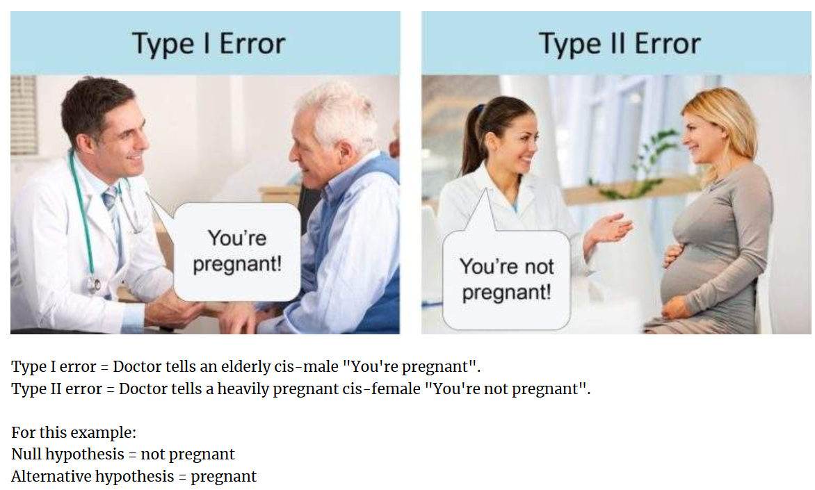
• Type I error = We reject the null hypothesis when the null hypothesis is true

• Type II error = We retain the null hypothesis when the null hypothesis is false

Null Hypothesis and the 2 types of Error example: Boy who cried wolf

Remember:

• Null hypothesis: No difference between groups. (the same)

  • H₀: Population mean 1 – Population mean 2 = 0. (H₀: µ₁ ‐ µ₂ = 0)

• Alternative: There is a difference between groups. (difference)

  • H_a: Population mean 1 – Population mean 2 ≠ 0. (H_a: µ₁ ‐ µ₂ ≠ 0)

Therefore our H₀ is that there is NO wolf. So Type I error occurs, when the true state of the Null hypothesis is TRUE (e.g. there is no wolf) but we reject the null hypothesis (thus we think there IS a wolf).

What is the usual value for a “p-value”?

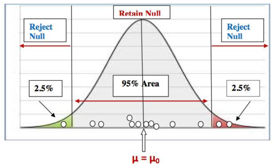
• The p‐value is normally 0.05. (Fits with 95% CI.)

  • This is the probability of a “Type I” error occurring

• If the p‐value > 0.05

  • Insufficient evidence to reject the null hypothesis

  • Thus “do not reject” or “retain” the null hypothesis

  • DO NOT say “accept” the null hypothesis!!

  • If the sample mean falls within 95% of the middle area, then we say that it is close to the population mean under the null and any differences between sample mean and null hypothesized population mean is due to sampling variability or by chance

• If the p‐value < 0.05

  • The probability that an observed result of big (or more) occurring due to chance is small

  • Thus sufficient evidence to reject the null hypothesis

  • We reject the null hypothesis (no difference), and accept the alternative hypothesis (there is a difference)

  • If the sample mean falls either in the lower 2.5% area or in the upper 2.5% area, then we say that the sample mean is so far out that a sample mean this large would rarely occur just by chance when the null is true

  • So we will conclude that the sample data does not support the null hypothesis and we go with the alternative hypothesis

Hypothesis Tests - What do P-values even mean?

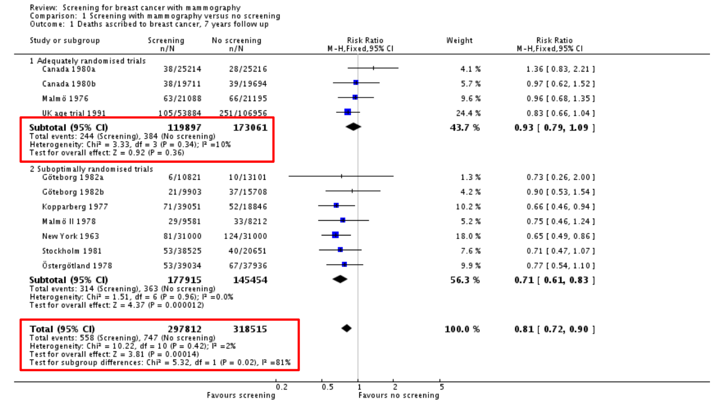
• Adequately randomised trials, p = 0.36

  • 36 out of 100 times, an observed effect being this big or more, is due to sampling variability or by chance

• Overall effect, p = 0.00014

  • 14 out of 100,000 times, an observed effect this big or more, is due to sampling variability or by chance

  • This means there is more likely to be a true difference

  • The study result is so rare that a chance factor can be ignored for the difference from the hypothesized value

What are the steps in Hypothesis testing?

• State the study

  • Summarise the study objectives (its importance and implications in public health)

  • State the study type

  • Write down the information you have (sample size etc.)

• 1) State the hypotheses

  • Null (no diff), Alt (diff). One or two‐sided? Justify

  • justify your selection of alternative hypothesis

    • For example, if you are considering a two-sided alternative hypothesis, provide evidence that supports your choice

• 2) State the assumptions & check them

  • Data should follow at least approximately normal

  • Patients in the sample should be selected randomly

  • Patients within a sample should not be related (or should be independent)

• 3) Analyse the data

  • Use the most statistical method to evaluate the hypothesis

  • Obtain the Test statistic value & p‐value (manual or software)

  • Calculate the 95% confidence interval too

• 4) Discuss the results & make an inference on the population

  • Discuss the summary statistics

  • Are the results significant or not?

  • Make an inference/conclusion on the study population

What are the types of tests (means)?

• One‐sample mean

  • Rare test in “real life” research

  • This is when you test one sample’s mean against a mean that you think it will be

• Difference between means

  • Large samples or known population SDs

  • Its rare the population SD is known and the mean is not!

  • Small samples, equal SDs — Far more common

  • Small samples, unequal SDs

• Mean of differences

  • Paired measurements

What are the 3 methods to test whether the SD is equal or unequal?

The formulas for SE and df for “difference of two means” is different for equal and unequal SDs

Method 1: Present the data graphically (histogram or boxplot)

• Compare the dispersion (spread) of the two groups

• If the spread of the data in each group is similar, assume equal SDs

Method 2: Calculate the ratio of the variances

• Note: Variance = SD²

• If the ratio < 2, assume equal SD

• If ratio ≥ 2, assume unequal SD

• Formula is the image

Method 3: Use a statistical package

• Use a hypothesis test procedure known as the Levene’s test for testing the null hypothesis that the groups have equal variances against the alternative hypothesis that the groups have unequal variances

• If the resulting p-value ≤ 0.05, reject the null hypothesis, i.e., consider unequal variances.

• On the other hand, if the p-value > 0.05, retain the null hypothesis, i.e., consider equal variances.

Is the population SD known or unknown and finding the p-value

Testing for equal or unequal SD → Method 3: Use a Statistical package

• Graph Pad Prism (and other stats packages) assesses whether the SDs are equal or unequal as part of the analysis process

• Hypotheses associated with this check:

  • H₀: The two groups are equal SDs

  • H_a: The two groups have unequal (different) SDs

• How to interpret the results:

  • If the p‐value > 0.05, we do not reject the null hypothesis (i.e. We assume equal variances)

  • If the p‐value < 0.05, we reject the null hypothesis. (i.e. We assume unequal variances)

Wording:

• “The results are statistically significant” – when the p-value < significance level

• “The results are not statistically significant” – when the p-value > significance level

How to determine what type of tests to do?

Example 1: Birth Weights → Step 0: State the Study

• The birth weights of children born to 14 heavy smokers and 15 non‐smokers were compared. The sample was from live births at a large teaching hospital

• What type of study design?

  • Cross‐sectional if “snap shot” in time

  • Cohort if mothers followed up and birthweights of their child collected later

• Data available:

  • Birth weights born to heavy smokers

  • Birth weights born to non‐smokers

  • Birth weight is continuous

Example 1: Birth Weights → What Test to use? And is the variance equal?

• “Independent” → can a mum be a smoker and non-smoker at the same time => NO, thus independent

Example 1: Birth Weights → Steps 1 Hypothesis & Step 2 Assumptions

• Null hypothesis: The population mean birth weight of babies born to heavy smokers and non‐smokers are the same

• Alternative hypothesis: The population mean birth weight of babies born to heavy smokers and non‐smokers is different

• Assumptions:

  • The two groups (heavy and non‐smoking) are independent

  • The mothers within each group are independent

  • The birth weight in each group follows a normal distribution (need to do the test - here we will just assume it is normal)

Example 1: Birth Weights → Step 3 Calculations

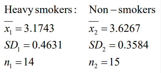
• Collate the information you have (image above)

• Calculations needed for the hypothesis test and 95% CI as followed in the image below

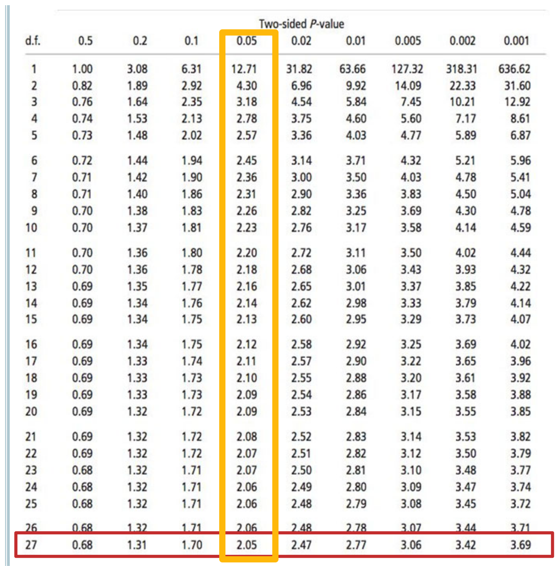
Example 1: Birth Weights → How to calculate T-multiplier?

• df = 14 + 15 - 2 = 27

• 95% CI means two-sided p-value is 0.05 (depicted in image above - two sides of the curve with 2.5%)

• T mult = 2.05

Example 1: Birth Weights → Calculate SE

Example 1: Birth Weights → Calculate the T-statistic

• Unpaired t-test → Independent t-test

• Look at 2-sided p-value

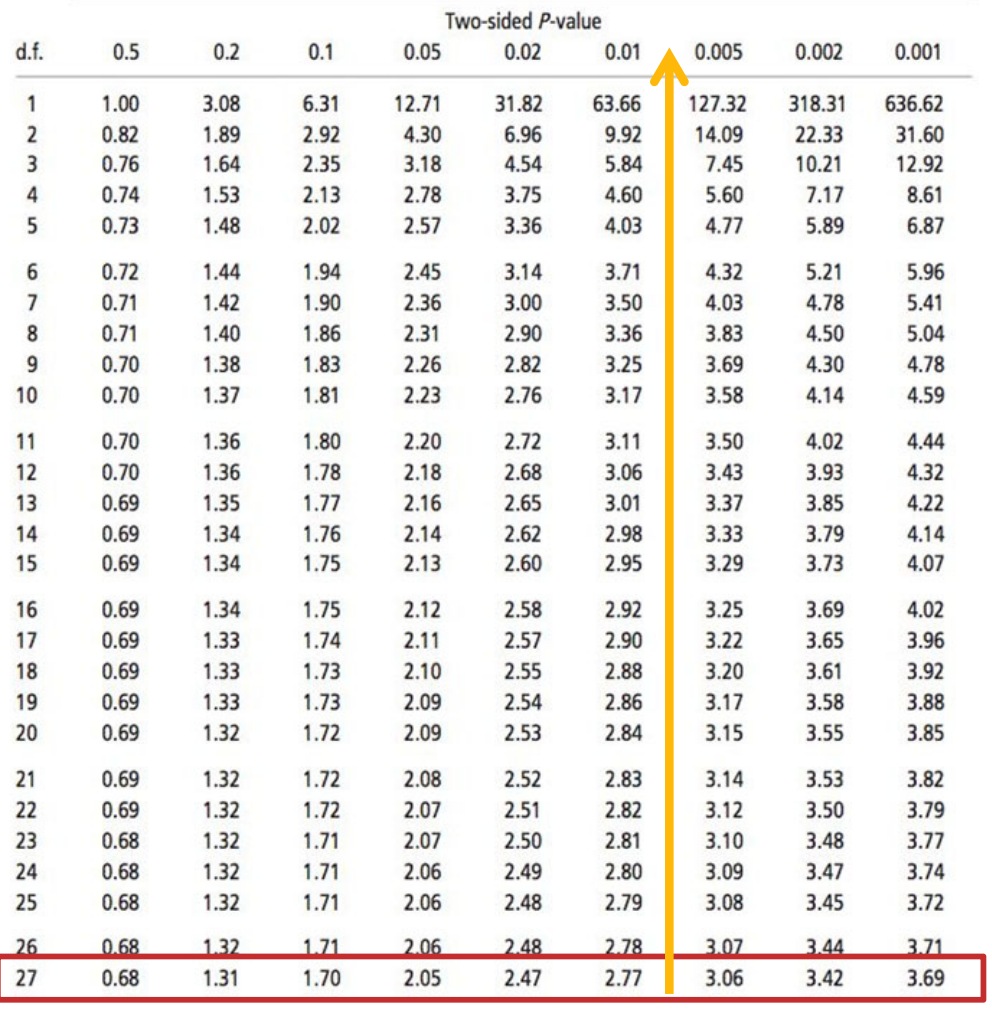
Example 1: Birth Weights → Calculate the p-value

• t‐statistic: ‐2.95

• p‐value is between 0.005 and 0.01

  • Note: A range is acceptable

  • A precise p‐value is obtained using a statistical package (see stats package videos for details)

• Interpretation:

  • The p‐value (between 0.005 and 0.01) is less than 0.05

• Decision:

  • Reject the null hypothesis (no difference)

  • Accept the alternative (there is a difference)

Example 1: Birth Weights → Calculate the CI

• We are 95% confident that the population mean difference between the birth weight of babies born to heavy smokers and non‐smokers falls between ‐0.77 and ‐0.14 kg

Example 1: Birth Weights → Step 4: Conclusion

• Report the means

  • The mean birth weight of babies born to smokers was 3.17 (± 0.46) kg and the mean of those born to non smokers was 3.63 (± 0.36) kg

• Report the CI and p‐value and comment on significance of the difference

  • The mean difference of ‐0.45 kg (95% CI of ‐0.77 kg to ‐0.14 kg [excludes 0]) and p‐value (between 0.005 and 0.01 [p‐value < 0.05]) allows us to reject the null hypothesis, providing evidence that the difference between groups is significant.

• Concluding remark giving the direction of difference

  • Hence babies born to mothers who smoked during pregnancy may have a reduced birth weight compared to those whose mothers did not smoke in the population

*In the end you should be able to write the conclusion without any headings

How to do the Two-Sample T-test for Unequal Variance?

What is the difference between T-multiplier and T-Stat?

Formula for an INDEPENDENT T-test - EQUAL SD

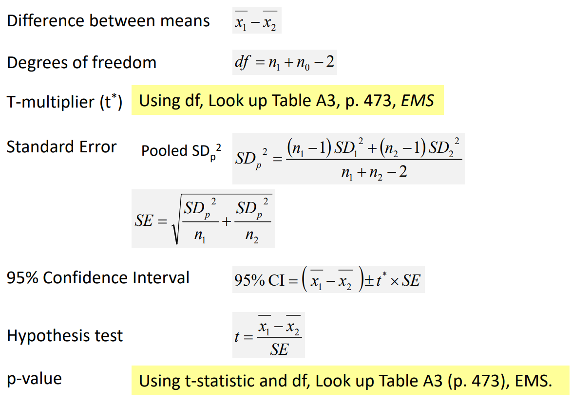
Formula for an DEPENDENT paired t-test