DAPAB W5L3: QTL analysis in biparental and multiparental populations
 Call Kai
 Learn
 Practice Test
 Spaced Repetition
 Match
 Flashcards
 Knowt Play
1/58

There's no tags or description
Looks like no tags are added yet.
59 Terms
Limitations in general quantitative genetics - before the era of markers
We could, using basic populations (P1, P2, F1, BC1, F2)
Estimate accumulated additive effects and dominance effects
Estimate H2, genetic variance - additive genetic variance
a,d,VA, VE etc
However, we could not:
Underlying loci responsible
idea about the nuber of loci or number of alleles involved
idea about their locationso n choromosomes
idea about the effect sizes of individual loci (importance of each)
idea about interactions with other loci (epistasis)
much informaition about linkage to genes for other traits 9postiive or negative)
QTL mapping in biparental crosses - schemativ overview
Parents pure lines, selfing species

QTL mapping in biparental crosses - schemativ overview
Parents heterozygous, outbreeding species
Sometimes called double pseudo-testcross
The idea
A QTl heterozygous in P1 can be mapped in the P2 background of the progeny: Qq: qq and vice versa
However, also QTLs heterozygous in both parents, Qq x Qq can be mapped (with less power, often)
For many ornamentals, trees (apple) and shrubs, many polyploids (Qqqq x qqqq) like potato etc

Mapping monogenic, qualitative traits
Add traits as a marker to marker data set
Linkage mapping can be enough
Sch loci mapped asif they were markesr
Using recombination frequencies
Monogenic resistance R/S
Some morphological traits: flower or fruit colour, shape etc
Mutations with large phenotypic effect: e.g. dwarfism, (male) sterility, vernalization requirements
QTL analsis also possible (and advisable)
assumptions not always correct

Mapping traits as single genes
Not possible in many cases
Some monogenic traits are not bimodal
Large environemtnal variation, two distributions overlap
Measured on a continuous scale with no obvious threshold
Many importatnt traits are quantitative and polygenic
Earliness, height, yield, partial resistance, quality traits, tolerance to abitoic stress
Solution: QTL analysis
What is a QTL, what is QTL analysis
QTL: Quantitaive Trait Locus
Region on a linkage group showing a statistical association iwth a quantitative phenotypic trait
Underlying QTLS: one or more genes
Each following Mendelian inheritance, single QTL can be explained by one or more genes
Region: confidence regions often large: 10-50 cM
Linkage group, markers and map used
Stastical association: stastical test procedure, statistically significant asosciation with trait
QTL marker linkage

QTL analysis - needed
Population segregating for markers and phenotype
Possible: selfed progeny of the mapping population:
Markers in the F2; trait in F3 lines (means per F3 line)
Genetic linakge map
Multiple- connected - populations possible too
Nested Association Mapping (NAM), MAGIC
NAM: one central parent crossed with a number of other parents
MAGIC: intercross, in consecutive generations of maybe 8 parents, until all are mixed, then selfed to become homozygous
Different ways of mapping QTLS
A statistical test per single marker
No map needed
Straightforward, basic statistical softwar suffices
But: power will decrease if marker - QTL more distant
Not every significant marker is a new QTL
Possible linked to same QTL - so map is useful even in this case
Interval mapping
Using adjacent markers for QTL analyses in the interval between them
Linkage map needed and more specialized software
Power higher than for single marker analyses
Multiple QTL mapping - composite itnerval mapping
Also allowing for QTLs elsewhere in the genome
Linkage map needed and specialized softward
Even larger power due to -
Test per marker
Two-sample T-test per marker
If only two marker classes
Anova
Any number of marker classes
Two for BC1, DH, RIL
Two or three for F2 (dominance, codominance of markers)
2,3, or 4 for F1 of outbred crop
Linear regression
on the #copies of a marker alle (0,1,2,)
Non-parametric test
Test of Kruskal-Wallis - using ranks of the phenotype
Two sample T test or Anova per marker

Statistical significance


Example: yield in barley DH: one chromosome
-10log (p-value)
threshold in red (p=0.05)
Five markers show significant difference
Evidence for one QTL on this chromosome
Plotted against map position
Tests only per single marker
Simple Anova/regression per marker
Significance expected for markers close to QTLs
Marker regression
If marker and WTL do not coincide exactly
QTL effects not exactly equal to differences between marker means
Effect could be larger if there are recombinations
Effect could be smaller too
What could be the effect of other QTLs
Power decreases with the effect size
Power decreases with the distance marker - QTL
Power decreases with higher random variability of the trait
Power can decrease with possible systematic variability due to presence of other factors in the experimetn
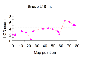
Per marker Anova, fruit flesh firmness apple
One threshold
Not a very smooth curve
Test: only available at marker positions
Gaps: non-infomrative markers
Signiciant region: end of chromosome 10
Assumptinos t-test and ANova
Normal distribution of the errors in the data
Indpeendence of the errors
Equal variance (Anova; t-test using pooled variance)
When can problems be expected?
If data are not continous but discrete (few classes)
If data are binary (0/1. present/absent)
If data are ordinal (visual scores on a scale from 1-5 for example)
If data are counts (number of pustules, nr diseased leaves)
If data are fractions of percentages
If strong outliers are present
If there are many values exactly equal (e.g. many zeroes)
F2 populations

F2 genetic model marker and linked QTL

F2 progeny

Model for the trait value resulting from a QTL

F2 progeny - table
D
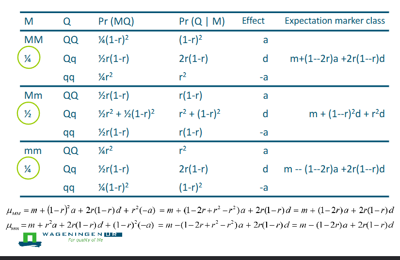
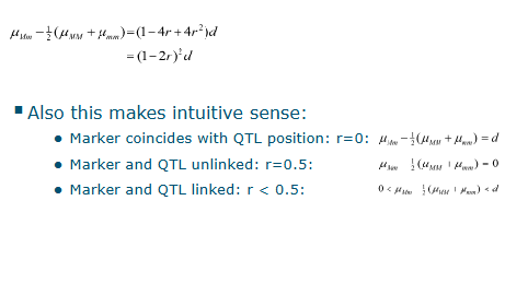
Difference between means of homozygotes
Difference depends on (confounded)
Additive effect of the QTL
Recombinatoin fraction between marker and QTL
Small difference:
Small additive effect of the QTL, marker closely linked
Large effect, but marker and QTL are more distat
Both needs to be estimated simultaneousy?

Difference heterozygote to mean homozygote
Factor influencing power of QTL analysis
Power of QTL analysis depends on:
Additive effect of QTL: aQTL = o.5(μQQ - μqq)
Dominance effect of QTL: dQTL: μQq- 0.5(μQQ + μqq))
Recombination frequency marker QTL: r
Remaining variance to the phenotypic trait
All other effects on the variance of the trait
Including possible other QTLs
In fact: standard error of differences between trait means marker classes
How to increase the power?
Contrast between the alleles should be large
Hard to influence - but maybe by choice of P1, P2
Contrast between the parentals if homozygous
Large segregation in the F1 if parents heterozygous
The size of the QTL mapping population
The number of markers
The trial in which the trait is evaluated
The quality of phenotypic scoes and marker scores
The chosen statistical analysis
Basic idea QTL mapping
As distance between QTL and markers becomes larger
Less information about QTL genotypes from markers
Smaller difference between marker genotype means
But:
Sometimes distances to another marker becomes smaller
Two linked maerks - a map
Possibel to use two markers flanking an interval on the map: interval mapping
Interval mapping
Consider positions between markers as possible QTL positoins
Pseudomarkers
Genotypes at the pseudomarker position estimated using
Map: distance between the (flanking) markers
Distance from the markers to the pseudo-marker
Genotypes of all idnviudals at those flanking markers

Interval mapping - two methods
Both methods:
Model observed trait values from unkoqn QTL genotypes and known marker genotypes
COmparison of a 1 QTL model with a no QTL model
So: a full model against a reduced model, F-test or likelihood ratio test
Method 1; regression on QTL probabilities - Haley Knott regression
Method 2; maximum likelihood approach
Build a probability model for the observations
Calculate likelihoods - assuming A QTL/NO QTL

Model phenotypic data (here in a BC1)
THERE IS A QTL (given markers m, rec. frequency r)


Model phenotypic data (here in a BC1)
THERE IS NO QTL (given markers m, rec. frequency r)

Which model fits the data better?
Histogram : observed phenotypic data
LOD score: log likelihood ratio

Interpretation of LOD score
LOD value of 10³ = 1000, 10log(1000) = 3
Likelihood of the data with a QTL 1000 times alrger than likelihood without a QTL
NO QTL: LOD close to 0
Note LOD for a QTL not the same as the LOD for linkage of a marker pair as used in linkage mapping
That would be 10log L(r=r_estiamted)/L(r=0.05=unlinked)
Example LOD score graph: firmness apple

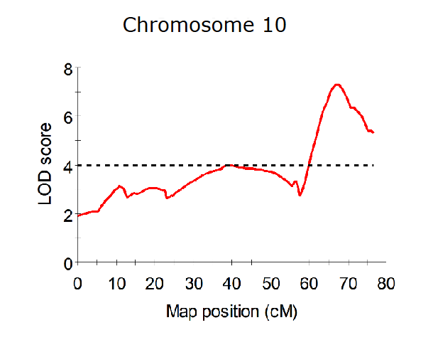
Need of a LOD threshold for significance
What should determine the threshold?
Pre-specified confidence level - 1-a (Often 95%)
Assumed data distribution, variance, etc
The number of tests
In case of multiple testing
Often: assuming independence of tests (Bonferroni)
QTL analysis:
Genome wide confidence level
Crop: number of chromosomes, size, marker density
Population (BC1, F2 etc)
Trait: not all have a known distribution
How to find a LOD threshold
Mathematical considerations
Population type, nr of chromosomes, total map length, marker density
Assuming normality of the trait
Simulated data
F2, BC1, DH, RILS, F1 of cross pollinator
Different chromsome lenghts and chromosome numbers
Assuming normality of the trait
Permutation of acutal data
Using the distribution of the actual data - no assumptino of normality
Results are often the same
Significance treshold
How many false positives are acceptable?
Per chromosome? Over the whole genome?
Many statistical tests
If we would accept 5% false positives per test
We do >500 tests we would expect >24 false positive results
However: tests on same chromosome not independent (linkage)
Trade-off?
Stricht threshold = high LOD threshold
Few fals positives (significance but no QTL)
More false negatives, lower power (no signicicane but there is a QTL)
Mild threshold - low LOD threshold
Fewer false negative results
More false positive results
Allow expected maximum of 5% false poitive genome-wide
Using simulatiions
SImulations
1.000.00 simulations
Fully informative markers - every 1 cM
Normal distribution of the trait
No QTL
1 chromosome
BC1, F2, RILS, F1 of cross pollinator (CP)
LOD score calculated every 1 cM
Per simulation highest LOD retained
Cumulative distribution of these LODs
Cumulative distribution maximum LOD

Calculation threshold
Genome-wide confidence - 95%
F2, 12 chromosomes, each 100 cM
Different chromosomes independent
First calculate confidence per chromosome
0.85^1/12 = 0.9957 -? 0.9956^12 =0/95
One chromosme, many simulations
Find, int he cumulative distribtuion: 0.9957
Read the corresponding LOD threshold
Table of cumulative distibution

LOD thresholds from simulations

Threshold: permutation approach
Idea
Reshulffle quantitative trait data creating random order
do this many times, e.g. 10.000 or more iterations
Retain the order of the genotypes for the markers
so, any relation marker/trait is broken
Per iteration
Perform QTL analysis
Retain maximum LOD of each chromosome
Retain maximum LOD over all chromosomes (genome-wide)
Give the distribtuion of these max LODS in a table
Read LOD threshold (like in previous case with simulations)
specific chromosome
genome-wide

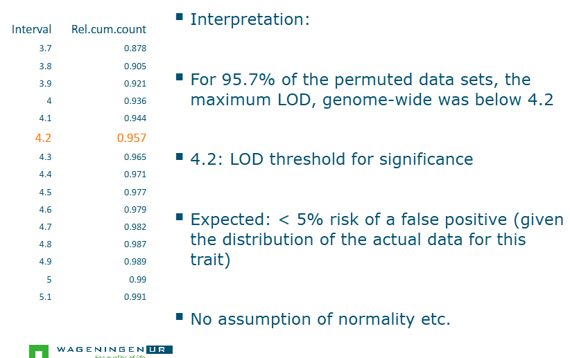
Permutation test: fruit flesh firmness apple: interpretation
Position of a QTL
Often very inaccurate - LOD peak is not at the gene
Resoltuion very low in biparental mapping populations
2-LOD support interval (fruit firmness)S

LOD support interval of a QTL
Often almost half a chromosome so poor resolution
It is not a 95% confidence interval
Rather an attempt to approximate that
2-LOD drop support interval often associated with about 95% probability to contain the QTL
under a lot of assumptions
1-LOD drop <95% probability
Works for single-QTL models in interval mapping, but not in multi-qtl appraohces with cofactors
Multi-QTL analysis (MQM or CIM)
MQM: multiple QTL mapping
CIM: composite interval mapping
Both based on same principle: correcting for other QTLs
Methods for QTL analysis
QTL analysis: analysis per single marker
QTL analaysis: interval mapping
by regression
By maximum likelihood
But:
= there may be more than one QTL (expected for many traits)
In the test only on eQTL at a time is accounted for
Problems
Low power if other QTLs are present (other or same chromosome)
Estimates QTL effects based
Ghost QTLS
one detected in the middle if more than one present on both sides
Undetected QTLs
Two QTLs can cancel each other out if positive allele linked to negative allele
Examle lower power
Two QTLs: one large effect, one small effect, markers exactly at the QTL position: demostration
Analyses:
Test for the small effect QTL, not taking into account hte large effect QTL
Test taking both markers into account

Example ghost QTL
Positive alleles of two linked loci are in coupling face
Coupling phase: the positive alleles are linke don the same homologous chromosome
Strongest effect could be obserrved in the middle instead of at either of the two true positions

Example two undetected QTLs
postiive QTL allele at the first locus is in repulsion phase with the positive QTL allele at the second
Repulsion phase: on different homologus chromosomes in a parent
Positive QTL allele at the 1st in coupling with the negative at the 2nd
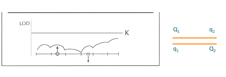
Multiple QTL analysis
QTL analysis with marker cofactors
cofactors absorb possible effect of QTLs elsewhere
AIM: enhancing power, decreasing bias
How to choose cofactors?
Many cofactors ovet the whole genome?
Near already significant markers?
Also some that are almost significant?
Pragmatic approach
Backward elimination from a user dfined set of cofactors
Cofactor seleciotn
Start: fairly large set of markers - potential cofactors
user defined, four or five per linkage group, included: makers with high LOD scores from interval mapping
Backward elimination procedure
Cclic approach,
Calculate likelihood with all selected cofactors
Calculate likelihood excluding one, do this for all
Drop marker with the smallest, and non-significant change
Continue dropping markers until change is significant
- Significant: dropping that marker would acuse a worse modle than the one before
Restricted MQM
MQM = mutiple QTL model
Restricted: considering cofactors on other linakge groups only
These segregate independently - statistically easy
Now: cofactors on same and other chromomes
same model everywhere, except fo rthe intervals that include a cofactor
More complicated analysis
- heavy computation, slower, dependence
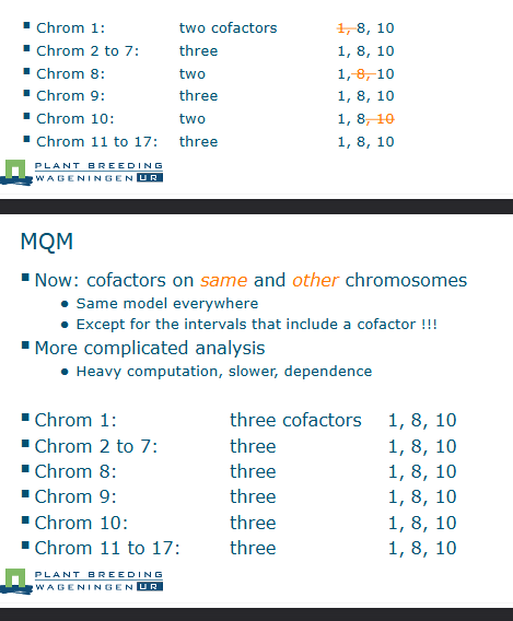
Apple fruit firmness: 3 cofactors, L10

More than one QTL on same chromosome
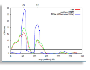
Summary QTL analysis
In single and multiple biparental populations or multiparental population
BC1, F2, RILs, DH, F1 (outbred), NAM, MAGIC
Three methods for QTL analysis
Premarker QTL analysis
INterval mapping
- with linear regression (-10log p-value)
with a maximum likelihood approach (LOD)
Multiple QTL analysis
Power considerations, issue of multiple testing
Finding a significance threshold