OLS Properties and assumptions

Set of Assumptions A1 (classical)

1- The observations {Yi, X2i, X3i, ..., Xki} for i = 1, ..., n are independent and identically dis-
tributed (iid)
2- E(u|X2, X3, ..., Xk) = 0
3- The variables {1, X2, X3, ..., Xk} are linearly independent.
4- V ar(u|X2, X3, ..., Xk) = σ2 (Homoskedasticity)
5- Conditional on {X2, X3, ..., Xk}, u is normally distributed.

Set of Assumptions A2

1- The observations {Yi, X2i, X3i, ..., Xki} for i = 1, ..., n are independent and identically dis-
tributed (iid)
2- E(u) = 0 and E(uXj ) = 0 for all j = 2, ..., k.
3- The variables {1, X2, X3, ..., Xk} are linearly independent.
4- Some moments of u and Xj are finite.

Properties of Estimators in General

Properties under the classical assumptions (A1) that require A1,2,3

The following properties require assumptions 1, 2 and 3
1. Unbiasedness: E( ˆβj ) = βj for all j = 1, ..., k.

Properties under the classical assumptions (A1)That require assumptions 1, 2, 3 and 4

Properties under the classical assumptions (A1)That require assumptions 1, 2, 3, 4, and 5

Assumptions	Result	Memory
1–3	E[β^]=βE[\hat\beta]=\beta	Unbiased
1–4	OLS is BLUE	Efficient
1–5	β^\hat\beta is normal	Normal
6	Estimate σ2\sigma^2	Sigma
7	t distribution	t-test

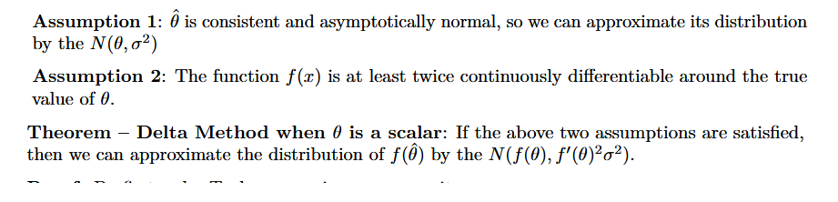
The Delta Method – for scalars Assumptions

The Delta Method – for vectors Assumptions

The Bootstrap method

The Jackknife method

Maximum Likelihood

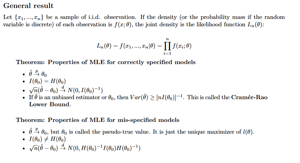
OLS is an MLE Estimator!

Generalized Linear Models

Logit and Probit Regressions

assumptions and properties understanding

Bias = centered?
Variance = spread?
MSE = bias² + variance?
Efficiency = lower variance?
Better = lower MSE?

A1–3 → unbiased
A1–4 → BLUE
A1–5 → normal
6 → estimate sigma²
7 → t

More error → more variance
More X variation → less variance
More multicollinearity → more variance

Heteroskedasticity → robust SE
Large n → consistency + normal approximation

One coefficient:

t=β^j−cSE(β^j)t=\frac{\hat\beta_j-c}{SE(\hat\beta_j)}

Then:

• Two-sided: reject if ∣t∣>1.96|t|>1.96 at 5%

• p-value < 0.05: reject

• Heteroskedastic: use robust SE

• Homoskedastic: classical SE is okay

• Fail to reject ≠ accept the null