Macro Lec 8

in the long run output is determined by

In the long run, output is determined by factor supplies and technology. 

Y bar

Y is the full-employment or natural level of output, at which the economy’s resources are fully employed. 

• “Full employment” means that unemployment equals its natural rate (not zero). 

basic short-run aggregate supply equation is 

where α is some number greater than zero, and EP  represents some expectation of the price level. 

This equation says that output may differ from its long-run natural rate if the actual price level turns out  to be different from the price level that people  anticipate. 

the most widely accepted explanation for an upward sloping SRAS curve

sticky price model

Reasons for sticky prices

• long-term contracts between firms and customers 

• menu costs 

• firms not wishing to annoy customers with frequent price changes 

assumption of the sticky price model

Firms set their own prices (i.e. firms have some market power)

How Firms Set Prices 

This price (p) depends upon two things: 

First, the general price level (P): think of the firm’s desired nominal price as depending on both the prices charged by its competitors  and the cost of its inputs. A rise in the general price level causes these to rise and induces the firm to want a higher price. 

Second, the firm’s desired price depends upon the level of demand  in the economy. Higher income raises the demand for the firmʼs product. Because marginal cost increases at higher levels of  production, the greater the demand, the higher the firmʼs desired  price.

We can summarize this as 

This equation says that the desired price p depends on the overall level of prices P and on national income relative to its natural level Y −Y bar

the parameter a measures

The parameter a measures how much the firmʼs desired price responds to national income. 

if output is at its natural rate

 If output is at its natural rate, then each firm’s optimal price is the same as the overall price level.  

When the economy is weak (output is below its natural rate), firms set their prices lower, and in a boom, when demand is high, firms set their prices higher. 

two types of firms in the economy

One fraction (1 − s) has flexible prices and adjusts its prices to  current economic conditions based on this equation.  

• The other fraction, s, is characterized by sticky prices. 

sticky prices

That is, due to the costs of price setting or some other reason, they set a price in advance and keep it in place for some period of time. They must set a price on the basis of expectations about future economic conditions. This involves forecasting both the level of demand and the price level. 

We will suppose that their best forecast about the level of demand is that it is at its long-run level. (This is consistent with the idea that there are random, unforecastable shocks to output that average out to zero.) Then firms with sticky prices just set 

p = EP

• That is, firms with sticky prices set their prices based on what they expect other firms to charge(other firms being their suppliers and competitors).

if output is at its natural rate, the actual and expected price levels correspond:

explain how  the actual price level equals the expected price level

 Sticky-price firms simply set their price equal to the expected price level, and 

• If output is at the natural rate, flexible-price firms set their price equal to the actual price level. 

high Y and high EP

• High Y → high P 

When income is high, the demand for goods is high. Firms with  flexible prices set prices high. [High demand causes flexible-price  firms to raise their prices.] 

• High EP →high P 

If firms expect high prices, then firms that must set prices in advance  will set them high. 

solving for the SRAS equation

the sticky price model says

The sticky-price model says that the deviation of output from the natural level is positively associated with the deviation of the price level from the expected price level.

The model says that output will deviate from the natural rate whenever prices exceed their expected level. 

• If the price level is higher than the expected price level, output  exceeds its natural level. If the price level is lower than the  expected price level, output falls short of its natural level.  

If P<EP

• Some firms change (lower) their price. 

• But many other firms want to avoid menu costs. So, they temporarily  lag behind in cutting their prices.  

• Because these lagging firms have prices that are too high, their sales  decline. 

• Declining sales, in turn, cause these firms to cut back on production  and employment. 

 If P>EP

• While some firms raise their prices quickly,

 • Other firms (strictly price firms) lag behind, keeping their prices low.  

• These low prices attract customers, inducing these firms  to increase employment and production. 

SRAS Curve

Note that the short-run aggregate supply curve is drawn for a given expectation EP and that a change in EP would shift the curve

Why the SRAS curve is convex 

• At low levels of output, there are lots of unutilized and underutilized resources available, so it is not terribly costly for firms to increase output, and therefore firms do not require a big increase in prices to make them willing to increase output by a given amount.  

•In contrast, at very high levels of output, when unemployment is below the natural rate and capital is being used at higher-thannormal intensity levels, it is relatively costly for firms to increase output further. Hence, a larger increase in prices is required to make firms willing to increase their output. 

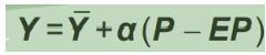
 three implications of this equation:

 First, the aggregate supply curve slopes upward. 

• Second, the position of the aggregate supply curve depends upon EP: the SRAS curve intersects the LRAS curve at a price level equal to EP, so a higher value of EP shifts the aggregate supply curve upward. 

• Third, the parameter α measures how much differences between actual and expected prices influence output. If α = 0, the aggregate supply curve is vertical; if α becomes very large, the SRAS curve is almost horizontal. 

what shifts the AD curve

• Changes in policy (fiscal; monetary) 

• Shocks to the money and goods markets. 

what shifts the AS curve

• Long run AS – changes in factor supplies, in technology 

• Short run AS – the above, plus changes in expected price level. 

• But note: Expectations change over the long run: if people observe that the price level is different from what they expected, their expectations adjust and the shortrun aggregate-supply curve shifts. 

• In the short run: expectations are fixed and the economy finds itself at the intersection of the AD curve and the SRAS curve

steps

Initial equilibrium 

1.Start at Ybar = Y₁ and P₁. 

AD increases unexpectedly. 

2.Then there is a positive AD shift, which shifts AD₁to AD₂. 

3.The shift then results in a new short run equilibrium at Y₂ and P₂, the intersection of AD₂ and SRAS₁. 

4.The price level adjusts. 

5.The price level adjustment shifts SRAS₁to SRAS₂. The new long-run equilibrium is at Ybar=Y₃ and P₃.  Here, LRAS, SRAS₂, and AD₂ all intersect. 

unexpected shift in the short run

The unexpected shift happens in the short run after firms set their prices based on what they expected, it could be that policies change or that a variable like consumption or investment demand shifting, output now rises above the natural level, the price level doesn't adjust immediately so it's above the level that the sticky price firms expected

changes in the expected price level

Changes in the expected price level shift the SRAS curve (this should be clear from the equation, as should be the fact that a change in the natural rate of output will shift the SRAS curve). Now that these new firms have higher prices and are responding to the higher demand, these firms with the lower prices are able to attract more customers so they also add to the  increase in output/income, causing it to rise above the natural level, if output is increasing then unemployment is likely going down so firms would hire more workers so the economy can now produce the non natural level 

Shifts in Aggregate Supply 

• An event unexpectedly changes firms’ cost of production (eg: an  oil price shock) 

• There will be a shift in the SRAS (eg: higher production costs  reduce profitability and therefore quantities supplied; SRAS shifts  to the left)

summary of sticky price model in one sentence

 It implies that output rises above its natural rate when the price level rises above the expected price level.