Stats 2

Types of variables

nominal (categorical with no ordering), ordinal (categorical with ordering), continous (interval or ratio) and discrete

Symbols

see image

Covariance

variance between two random variables, is unstandardised (not all variables are measured on equal scale), doesn’t say anything about the strength

Correlation (calculated through Pearson’s r)

standardised version of covariance, range from -1 to 1, < 0.1 is very small, 0.1-0.3 is small, 0.3-0.5 is moderate, 0.5-1 is large, 0.33 is sufficient enough association

Assumptions of Pearson’s r (correlation)

both variables must be continuous, linear + monotonic relationsip

Spearman’s Rho

for discrete/ordinal variables or non-linear graphs, does the same as r

Linear Regression (LR)

summary of the averages, tells us the best guess of one varibale when knowing the other

Linear model

y^ = b0 + b1 * x + ei, y^ is the predicted value, b0 is the intercept, b1 the gradient/coefficient, intercept shows us y^ when x=o

ei

the difference between our expectation of y and what y actually is

Ordinary Least Squares (OLS)

aiming for minimal errors when making a regression line, can be found through SS Residuals

SS Residuals (SSE)

sum of squared residuals, lets us find the graph with the least errors

Dummy variables

are either 0 or 1, if 1 the observation is party of the category, if 0 it is not (and part of another category)

Interpreting categorical IV

intercept is the reference category, for binary variables the coefficient will show one time changes, coefficients show the difference between the reference variable and the mean of the coefficient’s category

Who to choose for reference group?

binary variables don’t matter statistically speaking; for categorical varibales: avoid few observations, keep the order for ordinal or continuous variables, theoretical considerations

Calculating predicted values

see image

Issues & solutions ordinal IVs

OLS models assume the graph is linear which may not be true for odinal IVs, two possibilities: 1 treat the variables as categorical aka factorising them or 2 treat them as continuous only if there are enough levels >10

T-distributions

sampling a population a bjillion times and plotting the intercept and coefficient, we can use the estimated coefficient and SE to perform a hypothesis test using the t value, df and critical value (t > larger than critical value, reject H0)

Standard Error

how far does the sample mean differ from the population mean

Confidence Intervals

an upper and lower bound, the real value is likely to be within the bounds, if the CI does not contain 0 within the bounds it is statistically

Statistical significance

no significance doesn’t mean no effect just not rejecting null hypothesis, significance just means the null hypothesis can be rejected

Multiple Linear Regression (MLR)

includes multiple predictor (IV) variables, intercept is the expected value of y when all IVs are 0

Interpreting MLR

coefficients for continous variables mean the expected change in y if all other variables are held constant, coefficients for categorical variables mean the expected change in y when going from the reference category to the coefficient’s category

Standardisation of coefficients

we do this through calculating how many standard deviations each coefficient is from the mean, higher is stronger effect of the category

Confounding variables

an independent variable that affects both an IV and DV (size of fire (CV) affects both the number of fire trucks present (IV) and the amount of damage (DV))

Omitted variable bias

bias when an confounding variable is unaccounted for, what can we do: 1 randomising the values of the IV for our experiments 2 looking at natural experiments 3 statistical control → accounting for confounding variables

Post-treatment bias

controlling a mediating variable which leads to a reduction of the total effect

Accuracy of predictions

can be calculated through pearson’s r squared, 0 = no correlation and 1 = perfect correlation, important: adjust the r to account for multiple IVs

Issues with pearson’s r squared

can get a low value despite strong correlation if non-linear relationship, can get a high value while regressing IV on DV, can’t compare r squared with different samples, maximising r squared might not be the goal

SSR, RSS, SST

regression sum of squares, residual sum of squares (aka SSE), sum of squared totals

Model F tests

tests the difference between the model and a ‘null‘ model, if F value is above critical value then there is a (or more) statistically signficant IV

‘null‘ model

model with no IVs, all predictions are made with the intercept (mean)

ANOVA

analysis of variance, used to find the best fitting model, models should be compared in order of complexity

Interpretation of ANOVA

res.df = number of observations - IVs, df = how many more IVs this model has compared to the previous, pr(>F) = p-value (if this is smaller than 0.001 than the model is better than the previous one)

Linearity

assumption that our dataset is linear ‘enough‘, graphs should not be too non-linear

Residual plots

a new graph showing how far the residuals are from our predictions, if it looks random it is fine

Added-variable plots

shows every variable of a model independently, handy to check if a variable might be causing non-linearity

Solutions to non-linearity

making the mode non-linear to fit the data → using a polynomial function

Normally distributed errors

assumption that errors in our model will be normally distributed, can be observed through bell curves and Q-Q plots

Fixing non-normally distributed errors

changing the model’s contents, log-transform a skewed DV or use interactions

Homoskedasticity

assumption that there is equal variance amongst errors, can be checked through residual plots for funnel shape

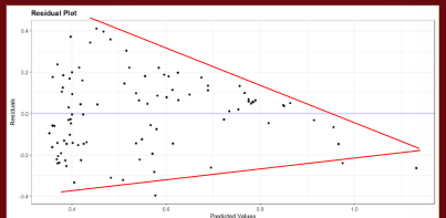
Heteroskedasticity

opposite of homoskedasticty, SE calculations will get screwed, can be fixed by changing the model specifications through using squaring (polynomial) or logging

Polynomials vs logs

best to use polynomial when the relationship is curvilinear and logs when the relationship is exponential/diminishing

Independent errors

assumption that our errors are independent, two ways of correlated errors → serial autocorrelation and geographical clustering

Serial Autocorrelation

when using last year’s errors can predict next year’s errors there may be a correlation, can be tested by the D-W statistic → outside of 1-3 signals autocorrelation

Solutions for autocorrelation

include a lagged dependent variable as predictor

Geographical clustering

when people from the same region are sample they might answer similarly due to socialisation

Solutions for geographical clustering

clustered standard error with fixed effects for cluster (or: making a bunch of dummy variables for all clusters), mixed/multilevel models allowing us to model variation both within and between clusters

Outliers

assumption that there are not too many outliers, we can see what an outlier is by calculating how many SDs it is away from the mean

Influential cases

can be investigated by Cook’s Distance, values above 1 are an issue, between 0.5-1 should be looked into, any deviating values should be investigated aswell

Solutions for Outliers and Influential cases

check for stupid mistakes, investigate the observations, do NOT remove them from the model (or communicate that you did)

Multicollinearity

assumption that our IVs are not linearly related to each other, makes it harder to identify the relationship between X1 and Y when X2 could also have an effect, can be identified through VIF statistic >5 is worrying and >10 very worring

Solutions to multicollinearity

create an index of X, usually try and live with it and contextualise your results

Perfect multicollinearity

X1 and X2 are perfectly correlated, can happen if variables are transformed versions of eachother (hieght in cm or inches) or happen through a dummy trap (not having a reference category)

Assumptions of OLS models

linearity, normally distributed errors, homoskedasticity, independent errors, outliers & influential cases, multicollinearity

Probability

proportion of times we see Y=1 relative to other possible outcomes

Odds

the ratio of the probability that something occurs compared to the probability it doesn’t occur, interpretation: >1 the probability of Y =1 is above 0.5 and <1 the probability is under 0.5

Linear Probability Models

linear models that work with probability, can lead to out of bounds predictions (0< or >1) and can be solved through using log-odds

Log-odds

the natural log (ln) of the odds, ranges from neg infinity to positive infinity

Interpretation of log odds

direction is easy to interpret, log odds = 0 then probability = 0.5, log odds >1 then probability >0.5, log odds <0 then probability <0.5

Odds ratios

tells us how much more likely in group 1 Y=1 than in group 2, can also be calculated by e^b where b = coefficient of the variable you want to calculate the odds of Y=1 (continuous variables intepretated as for every increase of X by how many odds of Y=1 increases)

Advantages of odds ratios

easier to interpret, an odd is unaffected by control variables

Disadvantages of odds

cannot know the absolute chances, people struggle to understand odds, difficult to understan total effect for continous variables

Predicted probabilities plot

graph of predicted probabilities, handy for marginal effects

Marginal effects

the average change in Y for every 1 point change of X, examples: OLS/AME/MEM, output is in probability points (if you times it by 100 you get percentage points)

MEM

maginal effect, takes the mode of control variables and uses them to make predictions in order to find the average, do not use this AME is better

AME

marginal effect, looks at every observation and uses its own combination of variables to average out all the values, used through newdata = datagrid in R

Z-value

tells us how ‘possible‘ the outcome of a probability model is, basically works the same as a t-value

CI for log odds

for odds ratios, instead of CI needing to not include 0 be statistically significant it needs to not include 1

Model fit of log models

best model fit according to maximum likelyhood estimation

Likelyhood

how well do the model’s predicted probabilities match observed data/outcomes, calculated through multiplying each predicted probability of their observed outcome

Log likelyhood

negative scale and closer to 0 means better model, calculated through R, LL

Null deviance

difference between null model and saturated model

Residual deviance

difference between our model and saturated model

Saturated model

model with perfect predictions

Likelyhood ratio tests

compares residual deviances between more and less complex models, models need to be nested, model that is closest to 0 is best,

Nesting models

creating sub-models, each including different combinations of predictor variables

Pseudo-r²

tries to do the same as r² but is not the same, used to analyse the strength between two variables when using log models

Assumptions of logistic models

linearity of the logit, independent errors of logistic models, multicollinearity, outliers & influential cases, complete seperation & perfect prediction

Linearity of the logit

assumes that changes in the logit are linear, can be checked through creating a scatterplot with a Loess line

Independent errors

same as OLS but we cannot use D-W test, to check use your knowledge of the study, fixed by clustered SE and multilevel models

Complete seperation & perfect predition

all values before a certain x are 0 and afterwards 1, can be seen through z=0 or p=1

Interacting effects

occurs when the relation between two variables is dependent on a third variable, best identified visually through a plot seperating the values of the third variable (aka making a graph for whites and one for blacks) or if b3 is not equal to 0

Interaction term (X3i)

multiplication of variables 1 and 2, its coefficient (b3) is found with the variable including a colon (:)

Interpreting interactions

1 identifying the ‘focal‘ variable and moderator variable (education level is focal and race is moderator, because education level depends on race) 2 correctly interpret the coefficient for the focal variable 3 interpret direction of coefficients 4 calculate predicted values and or marginal effects to get better interpretation 5 is the interaction statistically significant?

Interpreting direction of coefficients (interactions)

if both coefficients are positive the relationship becomes MORE positive BUT if b3 is negative the relationship becomes LESS positive, if both coefficients are negative the relationship becomes MORE negative BUT if b3 is positive the relationship becomes LESS negative

Marginal effects in interaction terms

calculated manually or via R

Statistical significance of interaction effects

Ho: the effect of the focal variable is homogenous (will not change if the moderater changes), if p < 0.05 we can reject Ho meaning there is an interaction effect

Considerations while calculating/interpretating interaction effects

all three parts are necessary to examine the interaction, will likely have high multicollinearity, precise measuring is difficult

Interacting effects with a continous variable

two issues: 1 what if the continuous variable cannot be 0 2 how can we effectively communicate when both variabes in the interaction are continous

Binary X Continuous interaction

the same as binary x binary

Continuous x continuous interactions

the same as binary x binary

Logistic models and interaction effects

same but few differences: 1 AME is more useful to interpret relationships 2 calculating the interaction term → odds ratios are multiplied instead of added (which i feel like you should do regardless????)