(3) precipitation

why measure precipitation?

to understand:

• historical average

• seasonal to annual

• or common period

of water cycle and its impact on the environment

what is a return period?

• used to estimate how much rain falling in a given time-period will produce stream flooding

• how long it will be between rainfall events of a given magnitude

→ streamflow & ppt relationship

types of rainfall ground-based measurements: rainfall

• manual gauges:

  • rainfall depth = (volume/area of orifice)

• tipping bucket gauge:

  • intensity of rainfall measured (number of tips)

• weighing gauge:

  • mass → volume (using density) → rainfall depth (mm) (using area)

  • converts the increase

  • con: wind

ground-based measurements: snowfall

• snow falling into gauge must be melted (be heated)

  • tipping bucket gauge:

    • heated shelter (e.g., propane)

  • weighing gauge or water level gauge

    • heated rim, storage reservoir filled with antifreeze

• snow/storm boards (NON MELTED)

  • accumulation of snow on board → snow depth = h₂

ground-based measurements: snow water equivalent (SWE)

convert snow depth → water equivalent using an assumed snow density (p_s): typically 100 km/m³
→ (snow has many possible densities → convert to standard (water depth)

!!! SWE = (p_s/p_w)h_2
→ (ratio of snow density & water density) × new snow depth

SWE → snow density (p_s)

SWE = (p₂/p_w)h_2
→ p_s = M_s / V_s

where:
M_s = mass of snow (kg)
V_s = volume of snow (m³)

= 𝛑r²h₂

→ typically 100 km/m³ (not always, not a constant)

SWE → density of water (ρ_w)

SWE = (p₂/p_w)h₂
ρ_w → constant = 1000 kg/m³

another way to find SWE using volume and area (ratio)

SWE = V_w/A_s

V_w = volume of liquid water (melted snow)
A_s = cross-sectional area of sampler

ground-based measurements: ultrasonic snow depth sensors

• measures total snow depth (H_s) by measuring time required for a sound pulse to reflect off the snow and return

  • how long a round trip takes

  • → measures how much snowpack grows

  • → use increase in H_s to determine h_s then estimate SWE

• then uses assumed snow density to estimate how much water that new snow contains

NON MELTED

ground-based measurements: types of error

• systematic: errors consistently in one direction; either over or under estimate (accumulate through time)

• random: errors unpredictably in either direction; tend to cancel out over time (over and underestimate)

ground-based measurements: wind effects

• change in turbulance

• wind more dangerous for snow

• snowfall much more sensitive (alters true measurements of snow catch as wind speed increases)

wind effect solution: wind shields

• calms particles around openings → allows to be more percise

• types of wind shields:

  • alter, nipher, combination, wyoming

ground-based measurements: other considerations/problems

• evaporation: water collected can evaporate before measured (underestimate) → add veg oil for protective layer

• wetting: some rainwater sticks to funnel surface due to adhesion (underestimate)

• measurement height:

  • lower gauge: less wind so more accurate but water can splash from ground in (overestimate)

  • higher gauge: less splash-in but stronger wind (underestimate)

• site characteristics

  • location of gauge → open area best

radar measurements of ppt

• emits electronic radiation with wavelengths in 1cm-10cm range

• waves are backscattered when they hit precipitation

• radar measures power of returning signal (& particle size)

• → allows for larger area

→ doplet size and ppt amount measured… intensity/speed of droplets

radar challenges

• Rain gauge bias: Errors in rain gauge measurements also affect radar accuracy when calibrating it

• Snowfall: Snowflake shapes vary, making snowfall harder to estimate than rainfall

• Melting snow: Melting snowflakes reflect strong radar signals, creating a misleading bright band

• Topographic obstacles: Mountains and other obstacles reflect radar signals, creating unwanted signals called clutter

ppt mapping methods (2)

• manual drawing of isohyets

• grid-based mapping

→ to visualize ppt distribution across an area

manual drawing of isohyets

contour lines → connecting points having equal ppt

→ assuming the same amount of ppt has fallen across a contour

grid-based mapping

• lay grid over area

• at each grid point, estimate ppt based on surrounding measurements

  • e.g., using inverse distance-weighted averaging → estimate ppt at each grid by combining measurements from rain gauges using weights, often giving closer gauges more influence

grid-based mapping (ppt) ex. PRISM

• displays pattern of ppt over large area based on topography → elevation alters levels

• higher elevations have better quality measured data cause less clutter and closer to satelite

what does point scale to distributed scale mean?

Using point measurements from individual rain gauges to estimate average precipitation across an entire catchment (distributed scale)

→ spatial integration of ppt covered next.. 4 methods

spatial integration of ppt

→ calculating actual average of ppt based on found measurements (averaging ppt accross an area)

• Arithmetic averaging: Average all rain gauge measurements equally (every gauge equal weight)

• Thiessen polygons: Weight each gauge's measurement by the area of its polygon.

• Isohyetal integration: Use precipitation contour lines and the area between them.

• Grid-based integration: Estimate precipitation at grid points and average them.

arithmetic averaging

• calculate average ppt by adding measurements from all rain gauges then divide by number of gauges

theissen polygons

divide catchment into areas where every point is closest to one particular rain gauge → estimating average ppt over catchment by weighting each rain gauge measurment according to area of its polygon

isohyetal integration

estimates average catchment ppt by weighting the average ppt between adjacent isohets by their area
Draw isohyets (contour lines connecting locations with equal precipitation).

• Calculate the average precipitation between each pair of adjacent isohyets.

• Multiply each average precipitation value by the area between those isohyets.

• Add the results and divide by the total catchment area.

what is an isohyet?

• line on map that connects points receiving the same amounts of ppt over a specific period

• help estimate average ppt accross an entire watershed

grid-based integration

estimates average catchment ppt by averaging ppt values estimated at grid points within the catchment → each grid point is given equal weight in the average

• Divide the catchment into a grid.

• Estimate precipitation at each grid point using nearby rain gauge measurements.

• Add the estimated precipitation values.

• Divide by the number of grid points to find the average.

→ use measurements outside of catchment boundary to calculate a normal ratio

point scale vs distributed scale

point: measures ppt at one location using rain gauge

distributed: estimates ppt across an entire watershed

→ why different?

• ppt varies between locations

• elevation, mountains, and storm patterns affect rainfall

• single rain gauge doesnt represent entire watershed

spatial variability in ppt

• Elevation: Precipitation can vary with altitude.

• Topography: Mountains affect precipitation patterns.

• Storm patterns: Some areas receive more rain than others.

• Wind: Can affect how much precipitation a gauge collects.

ppt significance

• driving variable of hydrologic cycle → input in waterbalance

• spatial and temporal variability of ppt reflect geographic variations in underlying processess

  • need qualitative understanding of underlying processes and resulting patterns

ppt requirements

• saturation of the air

• condensation (of water vapour to form ice crystals and/or droplets → condensation nuclei)

• growth of droplets to size sufficient to fall to ground level b4 evaporating

• continued input of water vapour to sustain process (depends on vertical wind and humidity)

SATURATION OF AIR

• add moisture to air

• cool air to the point of saturation

  • positive relationship of saturation and air temp

→ as temp increases, water held increases, saturation increases (warm absorbs)

saturation: how does uplift work as a cooling mechanism

• air parcel rises, pressure decreases → expands parcel and starts cooling

• for unsaturaed air: parcel cools at “dry adiabatic lapse rate” ~9.8°C/km

• once saturated → release of latent heat by condensation reduces rate of cooling

→ uplift towards cooler temps cools air/water vapour

→ warm rises above cooler air → difference in density (hot air balloon)

Why does uplift cause cooling?

Rising air experiences lower atmospheric pressure, so it expands and cools

→ Cooling increases relative humidity, but the air only becomes saturated when it reaches 100% relative humidity

uplift as a cooling mechanism: ways to saturate air

• convection

• convergence (non-frontal)

• convergence (frontal)

• orographic processes

convection

• warm, moist air rises

  • density of warm is less than of cold air → rises above (hot air balloon)

• sources of heat & energy: ground, sun, human activities (often driven by solar radiation)

characteristics of convective ppt

• mid-latitidues

• spatial pattern: scattered cells (in horizontal extent)

  • 1-10km

• minutes to an hour (relatively shorter)

• HIGH INTENSITY!

convergence (non-frontal)

• air moving via rotation of earth & etc. → air masses colliding

  • where do they go? → up (convergence!)

  • ex. tropical cyclones (hurricanes) from tropical zones → move towards land mass

→ intertropical convergence zone

convergence (frontal)

• extratropical cyclones

• cold front vs warm front

• convergence of different air masses from different climates FS

→ driven by different temp & density of air masses

• cold air pushes warm air up

orographic processes (5)

1. upward deflection: air forced over topographic barriers (pic)

2. orographic agumentation of other lifting mechanisms

3. frictional effects → increased duration of storms

4. topographic convergence

5. seeder-feeder mechanism
   
   

→ prevailing winds from ocean, air mass rises over hill, interacts with landscape → friction & slows → increased storm duration (slowed down)

orographic process 1

upward deflection: air forced over topographic barriers

orographic processes 2&3

ex. atmospheric river

• heavy rain/snowfall

• moisture originates from ocean (hawaii)

• convection/convergence → hit mountains (friction) → orographic

2. → this is the orographic augmentation of other lifting mechanisms

3. → friction increases storm duration

orographic process 4

4. topographic convergence

• landscape funnels air around/through channels → convergence

• stand-alone mountain range surrounded by water → moisture coming through pacific coast will move around mountain range then meets back together → convergence

  • moves around easiest path

orographic process 5

• seeder-feeder mechanism

  • blowing moisture into the air

CONDENSATION

• keep adding water to air for it to condense → cloud

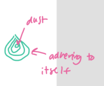
• condensation of water vapour to form ice crystals and/or droplets → condensation nuclei

  • clings onto other stuff in the air like ash, dust, soil

GROWTH

• growth of droplets to a size sufficient to fall to ground level before evaporating

  • existing water molecules run into one another (collision & turbulance) → grows then falls

CONTINUED INPUT

• cont. input of water vapour to sustain process (depends on vertical wind and humanity)

  • needs a source of water to continue (ex. into storm system)

spatial and temporal ppt are a function of what? (ppt patterns)

climate and topography

patterns in space and time (where and when)

• elevation variation

• rain shadow effect

  • dry part after moisture has fallen

• interactions between topography and weather systems

• lake effect

• seasonal variations

what is lake effect (ppt patterns)

• cold air masses pick up moisture and heat over warmer lakes

• friction and topographic effects of lee of lake create convergence → small scale atmospheric river