BIOL 251 Midterm 2

Life History

Life history: collection of age or stage specific traits directly affecting an individual’s reproductive success

Traits combine to make strategies that rep alternate trade-off solutions to the constraints faced by orgs.

Constraints: limitation to the possible types of life history a species can have in a given env

• ex. resources are finite, not all constraints are resource-related, constraints change w/ the env, and so the trade-off solutions differ by locaiton and over time

Life History Theory vs Strategy Vs Life Cycle

Life History Theory: Predicts how NS shapes the way orgs invest their resources into producing offspring to max fitness. There are trade-offs and optimization.

• Shared strategy connects individuals within a pop

Life History Strategy: pattern of heritable life-history traits that has evolved by NS over time in a pop in response to particular env conditions, depicted by life cycle

Life Cycle: series of stages that individuals go though in their life, from birth to death. Usually a circular diagram

• Many species alternate sexual and asexual reproduction (can be based on env cues)

Key Life History Traits

• Fecundity (potential reproductive capacity of an org)

  • High fecundity = lots of offspring (usually win against low)

• Longevity (average age achieved)

• Age at first reproduction (how long to reach sexual maturity)

• Adult size (how big to grow to reach sexual maturity)

• Degree of parental care

Investment in one life history trait increases, investment in another trait decreases - evolutionary tradeoff

Asexual Reproduction

Asexual: offspring are genetic clones of the parent. Does not contribute as much to genetic variation b/c no sexual recombo of DNA. i.e. fission, budding, parthenogenesis

Many invasives plates share life history traits that help them colonize new areas: asexual reproduction, clonal subsidy, wind dispersed seed and pollen, self-fertilization

Fungi have asexual spores (mitosis) and sexual reproduction.

Is favored when env are stable

Sexual Reproduction

Sexual: the product of meiosis and fertilization. 2 gametes = zygote

It is the most common form of reproduction in large, multicellular species. Greater genetic variation due to crossing over during meiosis and combo of parents gametes through sexual recombo.

Caused by a stressor or unfav conditions so it increase genetic diversity in which NS can act

Asexual vs Sexual Reproduction

Asexual - all offspring are genetic clones

• (+) high fitness under current conditions

• (+) rapid pop growth

• (-) low genetic variability - less adaptable to changing condition

Sexual - greater genetic variation in the pop

• (+) portfolio effect: genetic diversity min the volatility of the pop response to change in env condition

• (+) more raw material for natural selection to act on

• (-) takes time and energy if resources are scarce and the season is short

  • requires reproductive organs + courtship and mating (risky and use enegery)

Population Dynamics vs Demographic Parameters

Population Dynamics: study of the change in size of a pop through time

• depends on pop growth, dispersal, and demograhy

Demographic parameters: quantitative measurements of certain life-history traits that tell us about pop dynamics.

• Can vary by age → age specific values, can be represented in life table (per capita birth rate and per capita death rate)

  • Per capita = per individual in pop

  • i.e. birth and death

Per Capita Growth Rate - r

Key demographic parameters that influence per capita grow rate [r]

Ways pop shrink: death rate (d) & emigration rate (e)

Ways pop grows birth rate (b) & immigration rate (i)

r = b - d + i - e

• r > 0 → pop is growing

• r < 0 → pop is shrinking

• r = 0 → pop is stable (i.e. replacement rate)

NS optimizes demographic parameters to enable pop to persist in their env (r >= 0).

Note: diff demographic parameters can yield the same r but can diff in b and d rates through diff age structures

Demographic Pyramids

Age structures that tell the # of individuals at a specific age range. Differs from pop to pop.

Demographic pyramids have 4 shapes: rapidly expanding (high fecundity and mortality), slowly expanding, stationary (high fecundity and low mortality), or contracting (where mortality of young).

• ignore i and e

• include recent history (recent per capita b and d rates).​

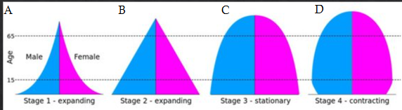
Life Table

Life tables summarize demographic parameters for a species or pop by age class (x). Summarizes the prob that an individual will survive and reproduce in any given year over its entire lifetime. Includes the probability of…

• Age specific births (b_x)

• Age specific Fecundity/reproduce (m_x = b_x / n_x)

• Age specific survivorship (l_x = n_x / n_o)

Survivorship x Fecundity = average # of offspring produced per female born

Dynamic vs Static Life Tables

Dynamic — track the survival of cohort though time → slow but accurate and fewer assumptions — very time consuming

Static — sample whole pop at a single timepoint → fast but assumes age specific demographic parameters are constant through time and age structure is unchanging. assumptions are rarely upheld — most common

Survivorship Curves

Survivorship is the proportion of individual remaining alive from one age class to the next

Plot survivorship curves: plots the # of survivors (y-axis and log) vs age (x-axis)

• Survivorship may be either the proportion surviving or the # surviving out of a n_o = 1000 cohort

• Helps recognize the general pattern of survivorship for a species or pop & compares to other pop or species.

Types of Survivorship Curves

Type I: high juvenile survival, high mortality at old age: e.g., dolphins, humans, elephants​ — high then low survivorship

Type II: mortality consistent with age, e.g. most birds​ — steady survivorship

Type III: high juvenile mortality, high survivorship in adulthood, e.g. trees, mussels, salmon​ — low than high survivorship

Net Reproductive Rate (R₀)

Net reproductive rate (R₀): average # of female offspring that each female has in a gen

• i.e. the # of offspring each individual in the pop has, on avg, before they die

• Ignore immigration

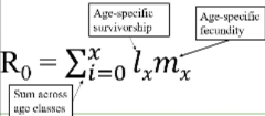
Generation Time (G)

The average age of a mother producing female offspring

Small gen time = pop will grow more quickly as their offspring will quickly replace them

Large gen time = pop will grow more slowly as female will wait till their bigger​

R₀ vs r

R₀ vs r vs G

r ~ ln(R₀) / G

• Increase R₀ = r increases and the curve gets steeper. ​

• Increase G = r decreases and the curve flattens out.​

Future Population Size N_t

Uses the exponential growth equation: N_t = N₀e^rt

• t is the # of years into the future

• N is pop size

Evolution of Life History Traits & Strategies w/ NS

A heritable life-history trait will evolve by NS when some variants have greater fitness than others.

Evolution by NS requires:

• Variation in life history traits

• That variation is heritable

• Some life history traits or strategies yield greater fitness for individuals (i.e. contribute more to the gene pool of future gen)​

The Principle of Allocation

The Principle of Allocation: any energy or resource an org uses for one function reduces the amount of energy or resource available for another function.

Limited energy: growth, maintenance, defense, reproduction/ reproductive effort

The cost to future reproductive success of the parent is in the form of reduced survival, fecundity, and/ or growth. Ex, Douglas fir trees produce more cones grow less in a given year

Current vs Future Reproduction

An individual’s reproductive effort should max its lifetime fitness

Optimal reproductive effort represents a trade-off b/w current and future reproduction.

• Allocation to current reproduction functions to increase current fecundity

• But reduce parental survival or growth, resulting in decreased future reproduction

• Survival, growth, and reproduction all contribute to fitness

Semelparous vs Iteroparous

Strat #1: semelparous is the # of offspring/ breeding event — one shot (i.e. salmo)

Strat #2: iteroparous is the # of breeding events — repeated reproduction (i.e. mammals)

Whether a species uses semelparity or iteroparity reflects its life history strat

Intermediate reproductive investment and iteroparity are favored where reproductive effort yields decreasing returns or parent’s mortality increases as the effort increases.

Otherwise, max reproductive effort and semelparity are favored

Number vs Offspring Size

Strat #1: generate lots of offspring, invest little in each w/ expectation of low survival rates. increase parental fitness but decrease fitness of young

• altricial: young born helpless

Strat #2: produce few young but invest heavily in each to max offspring survival. increase the fitness of young at the expense of fitness of parents

• precocial: longer gestation, young are born at a more advanced developmental stage

The production of altricial vs precocial offspring reflects a diff in life history strat

Number vs Offspring Size Conclusion

• If parental investment can improve offspring survival, precocial strategy is favored.

• If offspring survival is low despite parental investment, or it reduces parental fitness, then having altricial offspring is favored.

• If hatch rates are low but survival on hatching is improved by parental efforts, altricial makes sense

Current Reproduction vs Parental Growth

• NS will favor the age of maturity that results in the greatest # of offspring produced over the lifetime of an individual.

  • Usually, size is a function of age and food supply

• Reproductive effort increases w/ age b/c the # of future reproductive events decline w/ age

• If mortality increase after a particular age, reproductive effort increases before and decreases after that age

Red Deer

An example of current reproduction vs parental growth

• Red deer that had a baby (milk) have higher overwinter mortality than those that did not have a baby (yeld)

  • age related

  • declines in kidney fact due to energetic costs of lactation

• Milk hinders are also less likely to conceive the next year

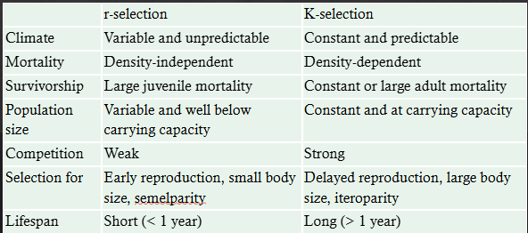
r vs K

There is a continuum in life history strats that seeks to optimize lifetime fitness for a species in a given env.

r (fast) → mature earlier, faster metabolism, higher reproductive output, fewer reproductive events

K (slow) → mature later, slower metabolism, fewer offspring . reproductive event

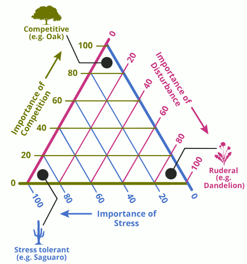
Grime’s CSR

The plant version of the r-K life history strategy theory

Competitor (C) (K - selected)

• Importance of competition

• Investment in resource use efficiency & individual seeds w/ later reproduction

• Typical of “good” condition

Ruderal (R) (r - selected)

• Grow fast, die young, lots of babies

• Important of disturbance

• Wide dispersal

Stress Tolerance (S)

• Importance of stress

• Low growth rate, long lived, high investment in defense

• Resistance to stressors

• Extensive storage of nutrients/ water

Winemiller & Rose

This focused-on life history of fish. Fish strategies could be explained by reproductive timing, juvenile survivorship, and fecundity.

Opportunities: reach sexual maturation fast and have small # of offspring. suitable to unpredictable env

• Importance of disturbance

Equilibrium: slow growth w/ later sexual maturation

• Important of competition & K-selected

• Few babies w/ high parental investment

• Type 1 survivorship, stable conditions

Periodic: slow to mature, but have lots of babies when they reproduce

• Importance of large-scale variability

• Type 3 survivorship

• Suitable to periodically fav conditions - long period of time

Population Growth

Population: collection of individuals of same species found at same time & place (so that they interact)

Population grows/ shrinks in response to changes in abiotic and biotic factors. i.e. food, spaces, resources, weather, interactions

Models are simplifications of complex things and are based on assumptions.

Models that are good enough can be useful as it tells which assumptions are no supported and where our understanding of a system is weak

Geometric Growth

Parameters: initial # and growth rate

Geometric Growth: discrete reproduction (reproduce at specific times) + unlimited resources

• Assumptions: non-overlapping gens (parents die before offspring reach maturity), resources are unlimited, and close pop (no i or e)

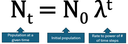
• Finite rate of increase (λ): ratio of pop size (N) at time t + 1 divided by N at time t in pop growing geometrically

• λ > 1 = growing, λ = 1 = stable, λ < 1 = shrinking

Pop size vs time is curved, pop growth rate vs size is linear, and r vs size is constant

Geometric Growth Equation

This is the generalized version to predict future N

Assumptions: non-overlapping gen (discrete reproduction) and no limits to growth: so λ can remain consistent regardless of N

Exponential Growth

Exponential growth: continuous reproduction + unlimited resources

• A differential equation, speed of growth: dN / dt

• dN / dt = rN

Per capita growth rate “r”: replacing lambda

• Assumptions: unlimited resources (r = r_max, or per capita = intrinsic rate of growth), no emigration or immigration (closed pop), and no crowding

Types of Growth Rate

Per Capita Growth Rate r: the per capita rate at which the population is currently growing

• dN / dtN, limited resources, actual measured speed

Intrinsic Growth Rate r: the per capita rate of growth for this species under ideal environmental conditions w/ unlimited resources.

• Max Intrinsic Growth Rate r_max: perfect ideal conditions + unlimited resources → declines w/ org size

Instantaneous Pop Growth Rate (dN/dt): the rate at which a population is growing at a specific point in time.

Human Population Growth

Humans are an ex. w/ exponential growth but we have raised our carrying capacity (max pop size that can be sustained in an env), but there are real limits to the human pop size we can reach and costs to other species on the planet

Logistic Growth

Logistic Growth: imposing limits

• Assumptions: resources are limited, continuous reproduction, and closed pop

• K: max pop size that can be sustained

• Growth of pop (# added per time step) is greatest in the middle

The rate of pop increase declines as you approach K due to density dependent factors, impact depends on pop size

Instantaneous pop growth rate is highest when N = K / 2

Density Dependent vs Independent Factors

Density dependent factors impact pop growth of both biotic (i.e. disease, parasitism, predation, etc.) and abiotic (i.e. food, space, nutrients, and water) factors.

Density independent factors impact pop growth through abiotic factors: weather, climate, pH, wind, natural disasters. It does not depend on pop size.

Logistic Growth Equation

b/c of density dependency, as you approach K, growth rate declines to 0, producing “S” shaped curve.

1 - N/K or (K - N) / K, determines if there is enough room to grow

So, when N = K, instantaneous pop growth rate (dN/dt) = 0, pop stabilizes

Logistic Growth

• Intrinsic rate of growth r is about biological potential to reproduce and is constant in exponential and logistic growth, dN / dt (speed of growth) is what changes

• Instantaneous pop growth rate (dN / dt) changes: largest w/ medium pop size

• Per capita growth rate (dN / dtN) changes: largest at small pop size, far from K

  • density dependent factors: less influence when far from K

Geometric vs Exponential vs Logistic

Pop size vs Time (N_t)

• Geometric & Exponential = curved

• Logistic = S-shape

Pop growth rate vs Pop size (dN/dt)

• Geometric & Exponential = positively linear

• Logistic = concave down (N = K / 2 is peak)

Per capita growth rate vs Pop size (dN/dtN)

• Geometric & Exponential = constant

• Logistic = negative linear

Dispersal

Real pop growth rate: r = b - d + i - e

Dispersal: permanent relocation & movement from one pop to another

• dispersal rates higher for patches closer together

• colonize newly available habitat

• can “rescue” pops from “extinction”

  • rescue: sink habitats receiving constant immigration from sources

i and e are related to dispersal and not the same as seasonal migration. Often in you adults and males seeking territories or joining other coteries/ herds/ etc.

Metapopulation

Pop in patches connected by dispersal can be considered a metapop. They are habitats in discrete patches

• occupied and unoccupied (extinct) patches

• Path occupancy (P): proportion of patches occupied

Even the largest patch has risk of extinction. Habitat patches are connected. Dynamic of the pop are not synchronous

The overall extinction rate (E) is proportional to the number of patches that could go extinct and therefore proportional to P

Classic Levins Metapop

The connections to prevent extinction. A metapop can persist even if none of the patches alone is big or productive enough to be a source habitat, providing:

• Habitat in discrete patches (Sources are always occupied and rescues the sinks)

  • Occupied and unoccupied (extinct) patches

  • Patch occupancy (P): proportion of patches occupied

• Even the largest patch has risk of extinction

• Habitat patches are connected

• Dynamics of the pop are not synchronous

B/c the pop dynamics in the discrete patches are not synchronized, there is enough rescue/ recolonization going on that the extinction of patches is offset and the proportion of patches occupied or the # of individuals in the larger metapop is stable

Patchy Pop

There is so much dispersal among the closely connected patches that their pop dynamics are synchronized and they’re effectively one big patch.

Conservation should focus on maintaining as large a cluster of patches as possible but there are also worries about disease.

Non-equilibrium metapop

Opposite of the patchy pop → dispersal among patches is too low and patches too isolated.

If certain links go extinct, the network can’t recognize and the whole metapop can go extinct. Conservation should focus on increasing connectivity among patches

Modelling Metapop Growth

Change in patch occupancy (P) can be modelled by logistic growth popualtion.

1. Extinction - more occupied patches (P) means more opportunities for extinction (e.g. due to disease)

2. Colonization

   1. Low (P) = low overall colonization/extinction rates as few numbers to spread

   2. Mid (P) = peak & most optimal

   3. High (P) = low overall rates as there are a few empty spaces

3. Equilibrium - when colonization and extinction meet

   1. Colonization > Extinction = P rises

   2. Colonization < Extinction = P falls

Metapop Growth Equation

• Metapop toward extinction: e / c > 1

• Metapop persist c / e > 1

Patch size and proximity determine c and e

• Size - larger patches lead to reduced extinction

• Proximity - nearer patches lead to higher colonization

Population Dynamics do not follow Models

Interspecific interactions can cause boom and bust pop dynamics that do not follow logistic growth

Variability in Pop

Environmental Stochasticity: “random” or unexplained env change

• density dependent & independent factors, abiotic, biotic

Demographic stochasticity: “random” outcomes of birth/death probabilities due to chance. stronger effect on small pop

• Allee effects: birth rate declines & death rate rises at low density creating an extinction vortex - small pops are more subject to extinction due to combined demographic and env variability

  • per capita pop growth rate at small pop sizes is lower than at high pop sizes

  • benefits of altruism and ease of finding a mate

Delayed Density dependency: a time lag between a change in a population's density and the effect of that change on its growth rate

Chaos From Deterministic Systems

• Unpredictable behavior even when underlying mechanisms is described

• Deterministic chaos: small diff in initials have a big effect later on, the butterfly effect

• Outcome is sensitive to initial conditions: a small change in one state of a deterministic nonlinear system can result in large diff in later state

e.g. discrete logistic models w/ time delay in the influence of density-dependent factors