Topic 6- Aggregate Expenditure Model

Aggregate Expenditure Model

the economy’s total level of output and income (real GDP) is determined by aggregate expenditures (or aggregate demand)

• focuses on short-run determination of total output (assuming price level is constant)

• developed by John Maynard Keynes

AE Formula

AE = the total planned spending in the economy

AE = C + IP + G + NX

4 Components of AE

• Consumption (C)- spending by households on goods/services

• Planned Investment (IP)- planned spending by firms on capital goods and by households on new homes

• Government Purchases (G)- spending on all levels of government on goods/services

• Net Exports (NX)- the value of exports minus imports

Planned vs. Actual Investment

• Planned Investment (IP)- what firms intend to invest and the inventory they expect to hold

• Actual Investment (IA)- what firms actually invest, including unplanned inventory changes

• the difference between actual and planned investment shows up as unplanned changes in inventories

Formula for Unplanned Changes in Inventories

Actual Investment - Planned Investment

Equilibrium

• occurs when actual investment = planned investment

• unplanned changes in inventories = 0

• spending on output = actual output produced

Equilibrium Condition

Aggregate Expenditure (AE) = Real GDP (Y)

Planned and Actual Spending Equations

IP = New Capital Stock + Planned Inventory

IA = New Capital Stock + Actual Inventory

When AE > Real GDP

• firms sell more than expected (shelves empty fast)

• inventories fall (actual sales > expected sales)

• firms increase production next period

• GDP and Employment increase

When AE < Real GDP

• firms sell less than expected (unsold goods pile up)

• inventories rise (actual sales < expected sales)

• firms cut production next period

• GDP and Employment decrease

Moving Toward Equlibrium

• if the macroeconomy is NOT in equilibrium, firms adjust level of production to move the economy toward equilibrium

• unplanned inventory changes tell firms if they produced the “right” amount or not

Aggregate Consumption Function

• shows level of aggregate consumption at each level of aggregate national income (real GDP)

• C = a + MPC(Y - T)

  • a = autonomous consumption

  • MPC = marginal propensity to consume

  • Y - T = disposable income

Autonomous Consumption

• the level of spending by households when income is equal to 0

• Y - T = 0

Disposable Income

• Disposable Income = Real GDP (Y) - Net Taxes (T)

• any disposable income NOT consumed by the household is saved

• Real GDP (Y) = Consumption + Savings + Taxes

Marginal Propensity to Consume (MPC)

• MPC = (change in consumption / change in income)

• AKA: change in C / change in Y

• slope of the AE Consumption function

• rate at which excess income becomes excess spending

Marginal Propensity to Save (MPS)

• MPS = (change in savings / change in income)

• AKA: change in S / change in Y

• MPC + MPS = 1

Factors that Effect Level of Consumption (6)

• Current Disposable Income- more income = more money to spend

• Household Wealth- rising asset values = more financial security/spending

• Expected Future Income- expected higher income = more willing to spend than save

• Price Level (average prices)- higher prices reduce purchasing power so consumers spend less (inverse relationship)

• Interest Rates- higher rates make borrowing more expensive and encourage saving over spending (inverse relationship)

• Taxes- higher taxes lead to less disposable income/spending (inverse relationship)

Investment (I)

• most volatile component of Real GDP

• adds to the nation’s capital stock

• Investment = Residential + Business Fixed (planned) + Changes in Inventory

Factors that Affect Investment (4)

• Expectations for Future Profitability- firms are more likely to invest if they expect high returns

• Interest Rate (nominal)- higher rates increase the cost of borrowing, making investment projects more expensive (inverse relationship)

• Corporate Taxes- higher taxes = lower profits = less incentive to invest (inverse relationship)

• Cash Flow (cash or liquid assets)- more internal funds makes it easier to finance investment without needing to borrow

Government (G)

• real government purchases include purchases at all levels of government: federal, state, and local

• spending is determined by policy and not driven by income

Taxes

• taxes collected by the government = T

• lump sum tax- does NOT change with income (fixed)

• proportional tax- varies with the level of income (Y)

Budget Deficit vs. Surplus

• deficit: G > T (government spending is greater than tax revenue)

• surplus: G < T (tax revenue is greater than government expenditures)

Factors that Affect Net Exports (3)

• Price Level (in the US vs other countries)- if US goods are more expensive, exports go down and imports go up

• Growth Rate (in the US vs other countries)- higher growth in the US increases income/demand for imports, while foreign demand for exports may not rise as much

• US Dollar Exchange Rate- a stronger US dollar makes exports more expensive to foreign buyers and imports cheaper for US consumers

Autonomous AE

• spending that does not vary with the level of real GDP

• in the simple model, Investment, Government, and Net Exports are all autonomous

AE Equation

AE = [C (autonomous) + IP + G + NX] + MPC(Y)

Induced Expenditure

spending that varies with the level of Real GDP

AE Model on a Graph

• 45 Degree Line- shows all points where planned aggregate expenditure equals real GDP (Y = AE)

• Autonomous AE- level of spending when real GDP = 0

• Equilibrium- occurs where the AE line intersects the 45-degree line

Slope of the AE function

• Slope AE = (change in aggregate expenditure/change in income)

• AKA: (change in AE / change in Y)

• tells us the fraction of any change in real GDP that will be spent

• in the simple model, the AE slope is MPC

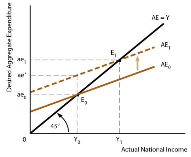
Parallel Shift in the AE Function

• the AE function can shift parallel to itself with a change in autonomous spending

• whole line shifts upwards, while the 45-degree line remains constant

• this shifts the equilibrium point to a higher level of AE and Y

Change in the Slope of AE

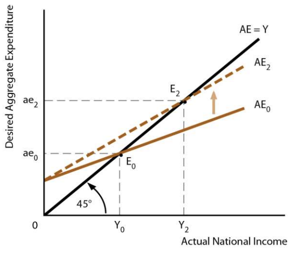
• results from a change in the marginal propensity to spend

• the AE line becomes steeper or shallower

• if the slope increases, equilibrium (where AE and the 45-degree line intersect) moves upwards and occurs at a higher level of AE and Y

AE Multiplier Effect

• a change in spending leads to a larger change in equilibrium GDP

• the change in equilibrium real GDP = the change in autonomous spending multiplied by the AE spending multiplier

• in reality, the size of the multiplier is around 2

AE Multiplier Formula

AE Multiplier = 1 / (1 - MPC)

Change in Real GDP Formula

Change in Real GDP = (change in AE) x (AE Multiplier)

More About the AE Multiplier

• the spending multiplier effect occurs both for an increase and a decrease in planned AE

• because the spending multiplier is greater than 1, the economy is sensitive to changes in autonomous expenditure

• the larger the MPC, the larger the value of the multiplier

• the simplified model omitts some complications (as real GDP changes, imports, inflation, interest rates, and income taxes change)

Aggregate Demand and Aggregate Supply

• the AD-AS model is used to analyze the overall production and price level of an economy

• helps economists understand how different economic events can affect the 3 macroeconomic goals (growth, unemployment, inflation)