Macro Lec 7

perfect capital mobility

Perfect capital mobility means there are no restrictions on the international flow of financial capital: The country’s residents can borrow or lend as much as they wish in the world financial markets; and because the country is small, the amount its residents borrow or lend in the world financial market has no impact on the world interest rate. 

Net exports, NX, are added to the goods market, which, combined with the assumption of perfect capital mobility, gives a new equation for goods market equilibrium, the IS* curve:

How NX depends on ε

 If ε is high, foreign goods are cheaper than domestic goods, so  consumers in the country will import more; exports would also fall. Therefore NX will be low. 

• If ε is low, the country’s domestic goods are cheaper, relative to foreign goods, so the country imports less and foreigners will demand more of its goods (i.e. the country exports more). Therefore the trade balance NX will be high

net exports function

The net exports function reflects this inverse relationship between NX and ε : 

NX = NX(ε )

mundell flemming model

 The Mundell–Fleming model assumes that both domestic and  overseas inflation are zero, and thus there is no difference between the nominal and real exchange rates. 

IS* curve

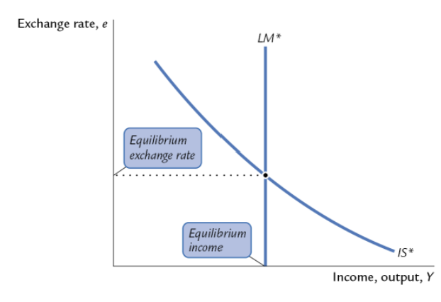
The IS* curve is now the combination of the exchange rate and  GDP consistent with goods-market equilibrium, given r = r*

a higher level of income leads to

Consider also, other things being equal, a higher level of income leads to higher saving and thus a greater supply of dollars to the foreign-exchange market. This leads to a fall in the exchange rate. The IS* curve thus slopes down.

Supply and demand in the foreign exchange market 

• Demand: 

• Foreigners need dollars to buy U.S. net  exports. 

• Supply:  

• Net capital outflow (S - I ) is the supply of dollars to be invested abroad

At the equilibrium real exchange rate, the supply of dollars available  from the net capital outflow balances the demand for dollars by  foreigners buying this country’s net exports.

 Two reasons why r may differ from r*

• Country risk: 

There is a risk that the country’s borrowers will default on  their loan repayments because of political or economic  turmoil. Lenders require a higher interest rate to compensate them  for this risk (risk premium). 

• Expected exchange rate changes:  

If a country’s exchange rate is expected to fall, then its  borrowers must pay a higher interest rate to compensate  lenders for the expected currency depreciation.

The LM* curve

• is drawn for a given value of r*. 

• is vertical because, given r*, there is only one value of Y that equates money demand with supply, regardless of e.

Equilibrium in the Mundell–Fleming model

 The equilibrium for the economy is found where the IS* curve and the LM* curves intersect. 

• This intersection shows the exchange rate and income at which the goods market and the  

money market are both in equilibrium. 

Note: In the small-open-economy model, the interest rate is fixed and the exchange rate can vary. In the closed economy, the interest rate can vary (and the exchange rate is irrelevant)

exogenous and endogenous variables in the mundell flemming model

The exogenous variables are fiscal policy G and T, monetary policy M, the price  level P, and the world interest rate r∗ . The endogenous variables are income Y and the exchange rate e.  

Floating and Fixed Exchange Rates

• In a system of floating exchange rates, e is allowed to fluctuate in response to changing economic conditions. 

• In contrast, under fixed exchange rates, the central bank  trades domestic for foreign currency at a predetermined price. 

Fiscal Policy under Floating Exchange Rates 

At any given value of  e, a fiscal expansion increases Y, shifting IS* to the right.  

• A fiscal expansion (increase in G or decrease in T) puts upward pressure on the country’s interest rate (shifts IS curve to the right). In a small open economy with perfect capital mobility, as soon as the domestic interest rate rises even the tiniest bit above the world rate, tons of foreign (financial) capital will flow in to take advantage of the rate difference.  

• But in order for foreigners to buy the country’s bonds, they must first acquire domestic currency. Hence, the capital inflows cause an increase in foreign demand for domestic currency in the foreign exchange market, causing the currency to appreciate.  

• This appreciation makes exports more expensive to foreigners and imports cheaper to people at home, and it thus causes NX to fall.  The fall in NX offsets the effect of the fiscal expansion.

In this open case, fiscal policy is ineffective in impacting output. When there's higher income from the fiscal expansion it pushes up money demand and interest rates. In the open economy when there is upward pressure on the interest rate, capital would flow into our country to take advantage of this higher rate. To invest in our country they must first have domestic currency, this increases demand for our domestic currency, this causes an appreciation of our currency, which causes NX to fall. 

• In a small open economy with perfect capital mobility, fiscal policy cannot affect real GDP.  

crowding out in a closed vs open economy

• Closed economy: 

Fiscal policy crowds out investment by causing the interest rate to rise. 

• Small open economy: 

Fiscal policy crowds out net exports by causing the exchange rate to appreciate.

Monetary Policy under Floating Exchange Rates

An increase in M shifts LM* right because Y must rise to restore equilibrium in the money market

• Initially, the increase in the money supply puts downward pressure on the interest rate. (In a closed economy, the interest rate would fall.) 

• Because the economy is small and open, when the interest rate tries to fall below r*savers send their loanable funds to the world financial market. 

• This capital outflow causes the exchange rate to fall, which causes NX—and hence Y—to increase.

Monetary policy, by contrast, is very effective under floating rates. The IS*–LM* diagram reveals that income rises and the  exchange rate falls.  

monetary policy in a closed and open economy

 Monetary policy affects output by affecting the components of aggregate demand: 

• closed economy: ⭡M → ⭣r → ⭡I → ⭡Y 

• small open economy: ⭡M → ⭣e → ⭡NX → ⭡Y 

fixed exchange rates

• Under fixed exchange rates, the central bank stands ready to buy or sell the domestic currency for foreign currency at a predetermined rate.  

• In the Mundell–Fleming model, the central bank shifts the LM* curve as required to keep e at its preannounced rate. 

 • The central bank must sacrifice control over the supply of money. Monetary policy now consists of adjusting the money supply such that the exchange rate is at its fixed level.  

• This system fixes the nominal exchange rate. In the short run, prices are also fixed, so a fixed nominal exchange rate implies a fixed real exchange rate as well.

Fiscal Policy under Fixed Exchange Rates

• Under floating rates, a fiscal expansion would raise e. 

• To keep e from rising, the central bank must sell domestic currency, which increases M and shifts LM* to the right.

Under floating rates, fiscal policy is ineffective at changing output. 

Under fixed rates, fiscal policy is very effective at changing  output.

Monetary Policy under Fixed Exchange Rates 

• An increase in M would shift LM* right and reduce e (dashed red line). 

• To prevent the fall in e, the central bank must buy domestic currency, which reduces M and  shifts LM* back left. 

• Under floating rates, monetary policy is very effective at changing output.  

• Under fixed rates, monetary policy cannot be used to affect output.

devaluation and revaluation of the currency

Devaluation is the deliberate lowering of a country's official exchange rate relative to a foreign currency or a basket of currencies. Revaluation is the deliberate upward adjustment of a country's official exchange rate by a central bank under a fixed exchange rate system.

Under a fixed exchange rate, the monetary authority however has the option of devaluing or revaluing the currency.  

• A devaluation reduces the exchange rate and shifts the LM* curve  out, implying higher income; the opposite is true of a revaluation

argument for Floating versus Fixed Exchange Rates

• Argument for floating rates: 

• allow monetary policy to be used to pursue other goals (stable  growth, low inflation) 

• Arguments for fixed rates: 

• avoid uncertainty and volatility, making international  transactions easier 

• discipline monetary policy to prevent excessive money growth  and hyperinflation 

the impossible trinity

Whenever you  choose to have free capital flow or free capital mobility there has to be a choice between having a fixed exchange rate and independent monetary policy. You can't have all 3, you have to choose 2. This is one of the implications that comes out of the mundell flemming model

• Option 1 involves allowing free capital flows and maintaining independent monetary policy but giving up a fixed exchange rate.  

• Option 2 entails allowing free capital flows and keeping a fixed exchange rate  but giving up independent monetary policy. 

• Option 3 is keeping monetary policy independent and fixing the exchange rate. Doing this requires limiting capital flows. 

Mundell–Fleming Model and the AD Curve for a small open economy

So far in the Mundell–Fleming model, P has been fixed. 

• To derive the AD curve, consider the impact of a change in P in  the Mundell–Fleming model.

 • We now write the Mundell–Fleming equations as: 

Note earlier , P was fixed, so we could write NX as a function of e instead of ε.  Earlier we wrote NX as a function of the nominal rate because the price level was  assumed fixed, so the nominal and real rates always moved together. But now,  with the price level changing also, we need to write NX as a function of the real  exchange rate. 

Deriving the AD Curve for a small open economy

 Aggregate demand is given by {P, Y} combinations such that the  foreign-exchange market and money market are in equilibrium.  

• As the price level decreases, the real money supply rises, and the  LM* curve shifts out. Equilibrium in the IS*–LM* diagram is thus  attained at a higher level of income. So the aggregate demand curve  slopes downward, as before.  

• The only difference is that the underlying reason is slightly different. In  the IS–LM model, a higher real money supply is associated with lower  interest rates, leading to higher investment. In the IS*–LM* model,  downward pressure on interest rates leads to a depreciation of the  real exchange rate that in turn encourages net exports.

Why the AD curve has a negative slope: (in terms of a small open economy)

• ⭡P →⭣(M/P) 

→ LM shifts left 

→ ⭡ε 

→ ⭣NX 

→ ⭣Y