econometrics 1 flashcards
 Call Kai
 Learn
 Practice Test
 Spaced Repetition
 Match
 Flashcards
 Knowt Play
1/100

There's no tags or description
Looks like no tags are added yet.
101 Terms
random variable
a function that maps random outcomes to real numbers
when X is discrete = discrete variable
when X is interval = continuous random variable
cumulative distribution function
gives the probability, for any real number x, that X is below x

probability distribution of discrete variable X
function that, for any real number x, gives the probability that X=x
probability distribution function (density) for continuous variables
denoted as f(x) and is the derivative of cdf F(x) at x

expected value (expectation/ mean)
E(x) of random variable X is the long-run average of X over many repeated trials
weighted average of all possible values of X

expectation is a linear operator
E(aX +bY) = aE(X) +bE(Y)
variance V(X)
the expected (squared) distance of X from the mean

variance is a quadratic operator
if a is a constant,
V(a)=0 V(aX)= a²V(X)
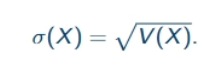
standard error
is the squared root of the variance
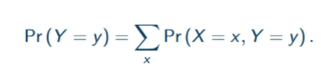
joint probability distribution of (X,Y)
characterised by the probabilities Pr(X=x, Y=y) for all possible combinations of values (x,y)
eg. P(Y=1)=P(X=0, Y=1) + P(X=1,Y=1)
conditional distribution
conditional distribution of Y given X=x is defined by:

bayes rule

conditional expectation
the conditional expectation of Y given that X=x is

conditional variance
the conditional variance of Y given X=x is:

law of iterated expectations (proof included)
for 2 random variables X,Y
E(Y) = Ex [ E(Y|X) ]
→ also works when conditioning on more than one variable E(Y)=E[ (Y| X,Z) ]

covariance ( and properties)
cov (X, Y)=cov (Y,X)
cov (a, X) = 0
cov (bX, Y) = b . cov(X, Y)
cov (X+Z, Y) = cov (X,Y) + cov(Z,Y)
cov( a+bX, c +dY) = b. d. cov(X, Y)

variance of a sum X+Y
V(X+Y)= V(X) +V(Y) +2cov(X,Y)
correlation
the correlation of X and Y can be defined by:

independence
two variables X and Y are independent when knowing the value of X foes not provide any information on Y. distribution of one variable doesn’t depend on realisations of the other variable

if X and Y are independent then:
pr(X=x, Y=y) = Pr(X=x) . Pr(Y=y)
E(X . Y)=E(X) . E(Y)
cov(X, Y) = corr(X, Y) = 0
V(X+Y)=V(X) + V(Y)
a continuous random variable X follows a normal distribution( gaussian distribution) when its density is:
where μ is the expectation, and σ² its variance
usually denoted as N (μ, σ²)

the normal distribution with zero mean and unit variance is denoted by:
N (0, 1)
its density is usually denoted as ϕ

normal distribution is symmetric around its mean
for Z normal with zero mean : p(Z > c) = p(Z < -c)
for the standard normal: 1-ϕ (c ) = ϕ (-c )

sample
is a finite collection of n observations of Y : {Y1, …, Yn}
→ is independently and identically distributed if:
for any i, Yi is drawn at random from the distribution of Y
for any i, j where i≠j, Yi and Yj are independent
sample average (mean) + properties
the sample average of a given iid sample is denoted as Ybar and given by
if Y is normal and the sample is iid, then Ybar n is also normal → as it is the sum of independent normal variables
Ybar n and its distribution can be approximated when n is relatively large using law of large numbers & central limit theorem

the expectation and variance of the sample average

law of large numbers
in an iid sample, Ybar n converges in probability to E(Y)
→ for any c>0, the probability that the distance between Ybar and E(Y) is larger than c, goes to 0 and n goes to infinity

the central limit theorem CLT
in an iid sample, Zn is asymptotically normal
→ for any z, P(Zn≤) converges to Φ(z) as n→∞
CLT also requires V(Y) must be strictly positive and finite
estimator
a random variable which is a function of the data sample
estimate
the numerical value of the estimator when computed on a specific sample
bias
when μ^ is an estimator of μ
bias: E(μ^) = μ
an estimator is unbiased if E(μ^) = μ
→ unbiasedness means that is we were to compute μ^ over many different samples, the average would be μ
consistency
μ^ is a consistent estimator is μ^ converges in probability to μ
→ having a consistent estimator in such a large sample means that the estimated value is probably very close to the true value
→ μ^ → p → μ for any c>0, the probability that the distance between μ^ and μ is larger than c goes to 0 as the sample becomes infinitely large
efficiency
μ^ is more efficient than μ^~ if V(μ^) <V(μ^~)
the values taken by the more efficient estimator tend to be less dispersed
confidence intervals
if b is a parameter and q a probability (often 95%). the q confidence interval for b CIq(b) contains the true value of b with probability q
→ it’s the set of values b* that we could accept b=b* against b≠b* at the 1-q significance level
in practice with an unbiased and (asymptotically) normal estimator b^ of b:

p-values
the p-value of a test is the largest significance level at which we could conduct the test and still fail to reject Ho
p-value = P Ho[ |T|>|t| ]
T is the test statistic, t the realisation in the data sample
if the probability is small this value of T is unlikely so we can reject Ho, if large then we cannot
matrices
a matrix M size (r, c) with r rows and c columns
each element is denoted mij with i as the row number and j the column number
column and row vectors in matricies
a size (r,1) matrix is a column vector and a row vector is a (1, c) matrix
square matrix
has the same number of rows and columns : r = c
a square matrix M is symmetric if mij = m ji fir (i, j)
commutative
if a.b = b.a which is not true of matrix mutiplication and would only be true if one of the quantities was the identity matrix
transpose of a matrix
denoted as M’ or M^t
such that the kth row equals the kth column of M so if P=M’ elements pij = mji
when will a square matrix be symmetric
if M’ = M
→ original matrix equals transpose if its symmetric
transpose of a product
if the product MP exists then
(MP)’ = P’ M’
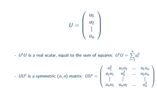
product of transposes
let U be a size (n, 1) column vector:
semi-definite matrices
a square (n, n) matrix M is positive semi-definite if there exists a matrix p with n rows such that:
M=PP’
→ we can think of PP’ as the ‘square’ of matrix P
invertability
a square matrix M (n,n) is invertible is there exists a square matrix, usually denoted M^-1, such that
MM^-1 = M^-1 M = In
if M is invertible, M^-1 it its inverse
if the inverse of a matrix exists, it is unique
if M and P are both invertible matrices, the product MP is invertible:
(MP)^-1 = P^-1 M^-1
linear dependence
a finite number of column vectors of similar size (r, 1) are linearly dependent if one of them can be written as a weighted sum of the other vectors
eg. A + B = 1 or A=2B
matrix rank / full column rank
the maximum number of columns of M that are not linearly dependent
if the rank of a matrix is equal to its column size the matrix is full column rank → if M is full column rank MM’ is invertible
eg. for A (m, n) rank A=n → full column rank
a square matrix is invertible if and only if it’s full column rank
random matrix
entries are random variables with a specified joint statistical distribution
the expectation E(X) of matrix X is the (n, K) matrix:

the variance-covariance matrix of a random vector (1, n)
V(Y) = E(YY’) - E(Y) [E(Y)] ‘
→ if α is scalar then V(αY) = α² V(Y)
→ if M is a deterministic/fixed (r,n) matrix (no random elements) then:
V(MY) = M V(Y) M’

SSR (sum of squared residuals) matrix
SSR(b) = (Y-Xb)’(Y-Xb)

OLS definition (matrix)
the sum of squared residuals SSR(b) is a function of parameter vector b
→ where solving this minimisation problem gives the expression of the OLS estimator

matrix OLS with one regressor (FOCs)
with matrix X and matrix b (1, 2) (containing only b0, b1)
the SSR becomes:
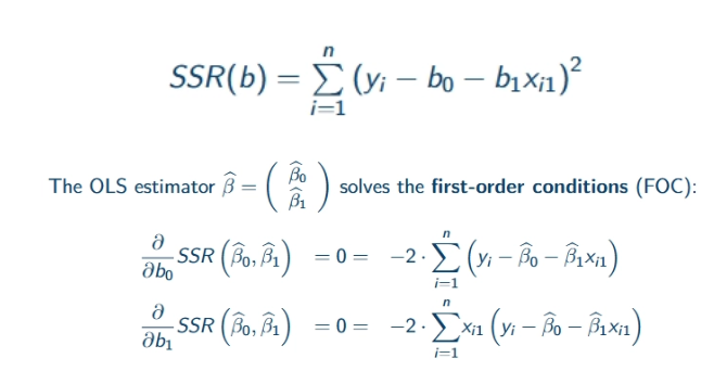
the expression of the OLS estimator (with covariance and variance)
using V^ (x1) = (x1²)bar - (x1bar)² and cov^(y, x1) = (yx1)bar-x1bar.ybar

matrix OLS with multiple regressors
OLS estimator β^ minimises:
then the FOCs rewrite as:
0=X’ (Y-Xβ^) → where the 0 is actually a (k+1) column vector of zeros
we than then solve for β^ → X’Y-X’Xβ^ = 0
X’Y=X’Xβ^
so, the OLS estimator equals:
β^= (X’X)^-1 X’Y

OLS existence and multicollinearity facts
OLS estimator exists if the system of FOCs admits a unique solution (invertible)
OLS exists if the matrix X’X is invertible
the square matrix X’X is invertible if matrix X is full column rank (the (k+1) columns of X must be linearly independent)
if these columns are not independent the regressors are multicollinear
predicted outcome in matricies
the predicted outcome is defined as:
yi^ = X’i β^
and the vector of predicted outcomes is

the vector of predicted residuals
the predicted residual is defined as:
ui^ = yi - yi^ → the error
the vector of predicted residuals is:

equation of how the predicted error is uncorrelated with any regressor

TSS (total sum of squares)
TTS is a measure of the dispersion of the outcome of interest
TSS/ (n-1) is the sample variance
using yi = yi^ + ui we have:

proof of the equality TSS = ESS + SSR
the last term equals 0 as we know the predicted outcome y^ and residual u^ are uncorrelated, and the mean u^bar of u^ is 0
→
0=cov^ (y^,u^)={sum to n} (yi^-yibar)(ui^-ui^bar)= {sum to n} (yi^-yibar)ui^ = 0

how to determine the fit of OLS (coefficient of determination)
the coefficient of determination is R²
R²=ESS/TSS = 1- SSR/TSS
the closer R² is to 1, the better the fit of the OLS regression
eg/ if R² = 0.2 → 80% of the change in Yi is coming from unobserved factors
exogeneity assumption
the exogeneity of the x variables:
E(u| x1, …, xk) = 0
as follows:
E(u)=0, E(u|xk)=0, E(uxk)=0, cov(u, xk)=0
proof of the exogeneity assumption
E(u)=0
E(u)=E[E(u|x1, …, xk)] = E[0] = 0
E(u|x1)=0
E(u|x1)=E[E(u|x1, x2, …, xk)]= E[0]=0
E(ux1)=0
E(ux1)=E[E(ux1|x1)]=E[x1E(u|x1)]=E[x1.0]=0
cov(u, xk)=0
cov(u, xk)=E(uxk)-E(xk)E(u)=0-E(xk).0 =0
moments conditions (2)
due to exogeneity and the solutions to the FOCs:
0=ybar-βo^-β1^x1^
0=(yx1)bar-βo^x1bar-β1^x²1^
we get the moment conditions:


OLS is unbiased in finite samples if
assuming an:
iid sample
no multicolinearity
exogeneity : E(ui|Xi)=0 for any i
a linear model: yi=X’i β +ui for any i
proof of unbiasedness

variance of the OLS estimator
the average of the square - the square of the average
V(β^| X)=E(β^β^’ | X)-E(β^|X)E(β^|X)’
and plugging in (from the image): we get the general expression for conditional variance of OLS→
V(β^|X)=(X’X)^-1 X’E(UU’| X)X(X’X)^-1

difference between homoskedasticity and heteroskedasticy
homoskedasticity: if all its random variables have the same finite variance
heteroskedasticity: if all random variables do not have the same finite variance
often occurs when there is a large difference among the size of the observations
→ eg. poor people will always buy cheaper food, but wealthy people with have more variance in eating both expensive and cheaper food
homoskedasticity
V(U|X)=σ²In
→ all error terms are not correlated (conditional on X) and they all have the same conditional variance σ²
combining exogeneity and heteroskedasticity we have:
E(UU’|X)=σ²In
plugging this into the OLS variance formula we get:
V(β^|X)=σ²(X’X)^-1
consistency of OLS → and what this means:
under exogeneity, OLS is a consistent estimator of β:
if β^ → p → β as β^ converges in probability to β
the probability there is a gap between β^ and β → 0 as n→ထ
the estimator of the constant converges to the model constant
βo^ →p→βo
for any regressor xk, the estimated coefficient converges to the causal effect:
βk^ → p →βk
asymptotic normality
an estimator that is asymptotically normal will have an approximately normal distribution as the sample size gets infinitely large
→ the distribution of an estimator becomes more normal as the n tends to infiinity
proof of asymptotic normality
from the proof of consistency we know (image):
where 1/n X’X converges to a matrix of expectations (not asymptotically normal)
and 1/n X’U is a vector of sample means
→ by CLT, each element of 1/n X’U is asymptotically normal
so β^ is a linear transformation of an asymptotically normal variable and is thus asymptotically normal
→ as a constant times a normal is still normal

when to use different tests (T or F)?
we can conduct tests on one parameter βk at a time→ T test
we can conduct tests on combinations of parameters → F test
T test example
consider a parameter in β: βk and a constant c →
test Ho: βk = c , Ha: βk
using the following test statistic (image):
the test statistic T and its asymptotic distribution are the same one sided vs. two sided
in a large sample , T is approximately distributed as a standard normal

F test example
testing on multiple parameters eg. Qβ=C where Q is a (q,k+1) matrix and C a (q, 1)
{ eg. βmale = 2βage}
test Ho: Qβ=C, Ha: Qβ≠C
the test statistic is:

internal validity of OLS (2 ways this can be violated0
the estimator of causal effects of interest may be biased or not consistent (exogeneity doesn’t hold)
the estimated standard errors may be inconsistent (sample not iid/ heteroskedasticity)
omitted variable bias
consider linear model y=bo + b1x1 + u
assume there is an unobserved variable x2 not included in y that is:
correlated with x1 and y
thus, it lies in the error term
u=b2x2 + ϵ where E(ϵ| x1)=0
OLS is thus biased and inconsistent for the causal paramter b1
if x2 is positively correlated with y → bias is positive, and y is overestimated, and vice versa
simultaneity/ reverse causality
Y could also have a causal effect on X
linear model: y=bo + b1x1 + u →
reverse causality arises from: x1 = ao + a1y + v (where cov(v, u)=0)
as x1 and u are correlated exogeneity is violated (image)

selection bias
arises when some data are missing as a result of a selection process that depends on Y, even after controlling for the regressors
→ Y= wage, x1=women yet not all women participate in labour market, so sub-sample of those who do may have different characteristics to the larger sample of the population , so the OLS estimate on the sample will be biased
can we regress OLS Y on a constant, m, x and x² ?
we can run such a regression as the relationship between age and age² is not linear so there is no multicollinearity issue, as long as age(or gender) is not constant in the sample
OLS fails if there is perfect linear dependence eg. if a²= c +da , as it would make X’X singular
eg. if a is constant at 30 (everyone in sample is 30) then age is perfectly collinear with the intercept. so OLS would fail because the regressors are no longer linearly independent
what does it mean if the OLS estimator is BLUE
this is the Gauss Markov theorem
BLUE stands for best (most efficient, lowest variance), linear (OLS is a linear transformation of the outcome vector), unbiased (the expectation of the OLS estimator is the vector of causal parameters)
under exogeneity and homoskedasticity, OLS has the lowest variance in the class of unbiased linear estimators
two properties for an instrumental variable to be valid
Instrumental relevance
cov(z, x) ≠ 0
z must be correlated to the endogenous explanatory variable x
Instrumental exogeneity
cov(z, u) =0
and must be exogenous in the linear model
setting up the instrument z with x
x = ao + a1z + ϵ
and predict
x^ = ao^+a1^z
two-stage least squares estimator 2SLS
if we have a valid instrument x we can use 2SLS , obtained by two consecutive OLS regressions
formula for t test in ols
T=(β-0) / SE
where SE = root var
F-statistic measures :
the relative increase in SSR per additional predictor, adjusted for the degrees of freedom
useful when testing the collective significance of related predictors x1, x2,… or dummy variables
null and alternative hypothesis in F-test
null hypothesis, Ho, states that the group of predictors tested jointly have no significant effect
eg. β1=β2=…βk=0
alternative hypothesis, H1, states that at least one of the predictors has a significant effect on the dependent variable
eg. at least one βi ≠ 0
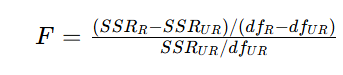
the test-statistic calculation in F-test
SSRr and SSRur are the sum of squared residuals for the restricted/ unrestriced models
dfr and dfur are their respective degrees of freedom
the critical value is determined by the chosen significance level (α) and the degrees of freedom
of the F-statistic exceeds the critical value, or p<α, the null hypothesis is rejected → indicating that the group of predictors jointly have a significant effect on the dependent variable
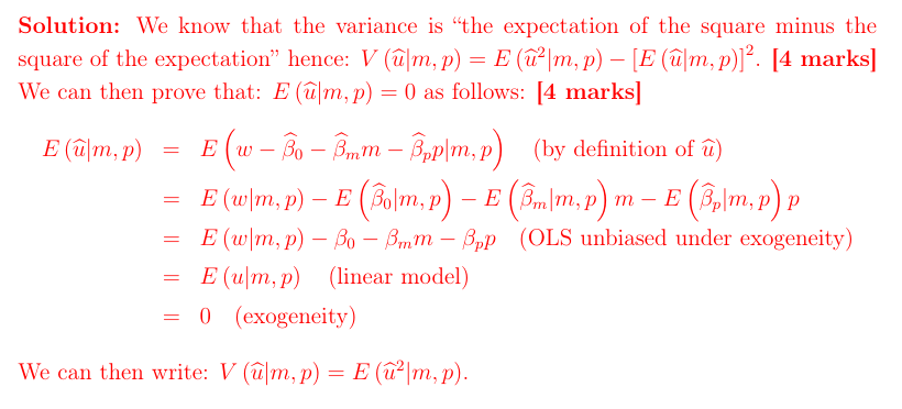
if u^ is the predicted residual, provde V(u^ | m,p) = E(u^²|m,p)
rewrite u^ as the fitted linear model of
then replace w with the linear model
using the exogeneity assumption that E(u| m,p)=0
show how testing for two slope parameters in this regression being jointly equal can inform on heteroskedasticity
an F-test will tell us if the coefficients of m and p are jointly equal to 0
if we reject Ho, either m or p has some impact on the squared precited residual [u^²=βo+β1x1+β2
first stage of the 2SLS
isolate the part of x that is uncorrelated with u. regress x on x using OLS
x = ao + a1z + ϵ
as x is uncorrelated with u, so its ao and a1z
yielding two-parameter estimates ao^, a1^, so we check instrument relevence : Ho ; a1 = 0 , H1: a1 ≠ 0
compute the predicted values of x (which captures the exogenous part of x), denoted by x^ as: x^=ao^ +a1^z
the only source of variation in x^ comes from z and is thus exogenous:
cov(x^,u)=cov(ao^+a1z, u)=a1^cov(z,u)=0
second stage of the 2SLS estimator
regress y on the predicted regressor x^ by OLS
because x^ is uncorrelated with u, β1 can be estimated by OLS
we look at how y responds to exogenous changes in x^
→ this can be interpreted as a causal response
the resulting estimator is the two-stage least squared estimator

consistency of the 2SLS estimator
y=βo +β1x+u
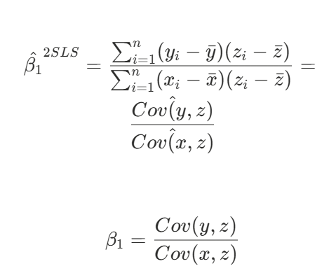
we can rewrite β1 in terms of population moments:
cov(y,z)=cov(βo+β1x+u, z)=β1cov(x, z)
where cov(u,z)=0 due to instrument exogeneity (yet if the instrument is not relevant, then β1 is not defined)
rearranging we can express β1 as
by the law of large numbers: the 2SLS estimator is consistent for β1 if z is a valid instrument for x:
B^(2SLS) → p → β1 (if either of the two assumptions needed for a valid instrument fails, the 2SLS estimator will not be consistent)
the 2SLS is not unbiased when:
x and u are correlated → meaning, when instrumental variable estimation is actually needed, the 2SLS estimator is essentially never unbiased
properties of the 2SLS estimator
if we have a large iid sample and a valid instrument, the 2SLS estimator β^(2SLS) has an approximately normal distribution
with mean β1, following from the consistency result
with a variance that has a (complicated) closed-form expression → statistical software will estimate the standard errors
alternative derivation of 2SLS estimator
start with y=βo+β1x+u , where E(u|x)≠0
use reduced form to relate y to z:
y=γo+γ1z+μ
the first-stage related x to z
x=πo+π1z+ε → where μ and ε are error terms, as we assume x is exogenous and uncorrelated with both
solve the first stage for x and substitute it in the reduced form
—> the effect on y of an exogenous change in x is β1=γ1 / π1 units

identification of the coefficients of IV regression
whether the coefficients are identified depends on the no. instruments (m) and the no. endogenous regressors (k)
so the coefficients β1,..,βk are said to be:
exactly identified: if m=k
there are just enough instruments to estimate β1,..,βk
overidentified: if m>k
there are more than enough instruments to estimate β1,…,βk
we can test whether the instruments are valid
underidentified: if m<k
there are not enough instruments to estimate β1,..,βk, if so, you need to get more instruments
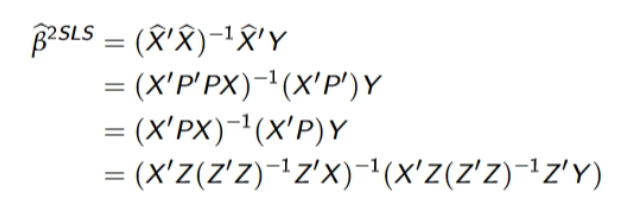
the 2SLS estimator in matrix form
we exploit the fact that P is independent and symmpetric so P’=P and PP=P
and X^=XP
showing that the 2SLS estimator is not unbiased in matrix form
Y=Xβ + U and plug it into the 2SLS estimator
to prove unbiasedness, we would need to show the last term is 0 in expectation
we would use expectations conditional on X, as under exogeneity E(U|X)=0
under instrument exogeneity, E(U|Z)=0 yet this is insufficient as the last term also involves the random variables X

our instrument is “strong” if
the F-test for it is larger than 10
instruments are weak if they explain very little of the variation in x, beyond the one explained by the w’s (included exogenous variables in z) → if all the π1,..,πm are either 0 or nearly 0
too weak correlation between x and z can cause the 2SLS estimator to have a large asymptotic bias even if z and u are only moderately correlated
2SLS will perform worse than OLS (will have a larger asymptotic bias) if:
