Unit 2.1-2.3 AP Statistics Quiz

10 matching, 8 mcq, 1 frq

Uni-variate Data

Data collecting observations on a single variable, so only 1 variable matters. Example: Hair color, height, gender, eye color

Bi-variate Data

Data collecting paired observations on 2 different variables, so 2 variables matter. Example: height and gender, hair and eye color

Qualitative (Categorical) Data

Data grouped into non-numeric categories or attributes. Example: Grades (freshman, junior) and zip code

Quantitative (Numerical) Data

Numerical measurements or counts, can calculate average. Example: length, width, psi, height, house number on a street

Discrete Data

Quantitative data taking on distinct, separate, or countable values. May be finite or infinite and whole numbers. Example: Y value in step function

Continuous Data

Quantitative data that can take on any value within a continuous range, measurable but not countable. Example: X value in step function.

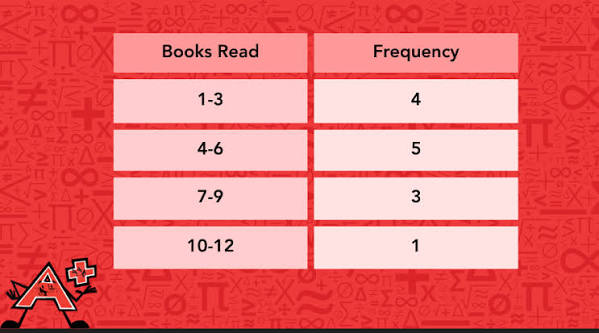
Frequency/Frequency table

Total count of occurrences for a specific value or category

Relative Frequency

The proportion or percentage of total observations belonging to a category.

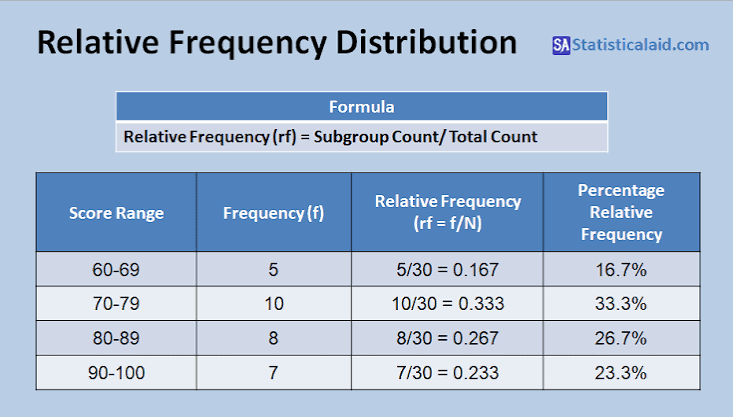
Relative Frequency table

Table displaying raw counts or relative percentages across categories

C.U.S.S (have labels)

C- Center (median or mean), U - Unusual features (outlier, gap, cluster in data), S - Shape (Way the graph appears: normal, skewed, uniform, [+,-]), S - Spread (How spread data is, usually range or standard deviation)

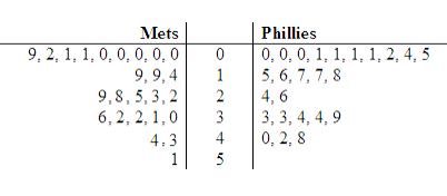
Stem and Leaf Plot

Splits quantitative data values int two distinct parts. Stem is leading digit, leaf is second or third digit, goes from smallest to largest on right side and largest to smallest on left.

Analyzing data

Minimum (lowest value in data set), Quartile 1 (# that marks 25% of data), Median (middle number of data), Quratile 3 (# that marks 75% of data), Maximum (high value in data set), IQR (Q3 #-Q1 #), something is skewed right is tail is on right side (vice versa for left)

Box Plot

Step 1: Do the 5 number summary (Analyzing Data), Step 2: Draw the box (middle 50%), Step 3: Whiskers (25% extension), Step 4: Outliers. If presented vertically, turn horizontally

Bar Graph

A visual representation of categorical data using rectangular bars proportional to frequencies or percentages.

Histogram

Graph that shows how quantitative (numerical) data is spread out and grouped across continuous ranges. To find the median in a histogram: Step 1 - Find halfway point between the frequency value or find the relative frequency of 50%. In picture it’s 31, so 31/2 = 15.5, so median would be between 75-80 feet. To graph a histogram: Step 1 - Find a good bin size (how wide), Step 2 - place each data point into bin, Step 3 - The number of data points in the bin corresponds to frequency

Pie Chart

Circular graph divided into proportional sectors reflecting relative frequencies

Area Principle

A data visualisation rule stating that the visual area occupied by a graphic representation must correspond directly to the proportion of data represented

Sample mean (x with the line on top)

The calculated arithmetic average of a subset/sample

Population mean

The true mean value across an entire population

Median

The middle value when data points are arranged in ascending order

Outlier

An extreme value that heavily influences the mean and standard deviation while having minimal impact on the median

Range

Total spread calculated as the difference between maximum and minimum values

Standard Deviation

A measure reflecting the typical distance or deviation of observations from the mean

Sample standard deviation (S)

Standard deviation computed using n - 1 degrees of freedom in the denominator

Population standard deviation (o or sx)

Standard deviation computed across an entire population

Unimodal

1 peak

Bimodal

2 peaks