Machine Learning 1 Exam

Statistical learning

the set of tools for estimating an unknown relationship between inputs and an output

Regression

Output is number on a continuous scale

Classification

Output is a category

Y=f(X)+ϵ

Y: output

X: inputs

f: true relationship (^f: estimated relationship)

ϵ: error term, everything that affects Y and is not in X, plus pure chance; deviation from true population line

Prediction

Accurate ^Y for new cases at the cost of knowing ^f

Inference

Understand how Y changes with X

Bias (Interpretable)

Underfitting (ex. linear regression); systematic error

Variance (Flexible)

Overfitting (ex. neural networks); sensitivity to the training data

MSE

1/n ∑y_i−f^​(x_i​))²

Gap between predicted an actual value, squared, summed, and averaged

• Squared: punishes big misses far more than small ones

RMSE

sqrt(MSE)

Predictions are off by the RMSE on average

Training error

MSE on training data

Test error

MSE on new data

Err(x)

Bias² + Variance + sigma²

Irreducible Error

randomness in the outcome itself

Supervised learning

A known set of predictors and response variables

Unsupervised learning

A set of predictors with no output, exploration of patterns

Clustering

Grouping by similarities

Dimensionality reduction

using PCA to compress and visualize high-dimensional data

K-Means Clustering

Measures distance between data; scaled so that every variable is on equal footing

Simple linear regression

quantifies the relationship between two numerical variables, one predictor and one response, to predict the response

• β0​ is the intercept

• β1​ is the slope

Residual

Gap between observed and actual value; deviation from the fitted line; unexplained variability

Intercept: Interpretability

• X = 0 is realistic

• at or near the range of your data

Slope: Interpretabilty

Each additional X unit is associated with a B1 increase/decrease units of Y, on average (holding other Xs constant)

Standard Error

how much the estimate would bounce around across repeated samples

Confidence Interval

If we repeated this sampling process many times, about 95% of the intervals we built would contain the true β1

t-statistic

counts how many standard errors the estimate sits away from zero

Hypothesis testing

H0: β1 =0

H1: β1 =0

Null: no true relationship between X and Y

p-value

the chance of seeing a t-statistic this extreme if the null hypothesis were true

Coefficient confidence interval

Where is the true slope?

Confidence interval for the mean response

Where is the average outcome for all cases with these predictor values?

Prediction interval

Where will one new individual outcome land? Carries true error on top of estimation uncertainity

Residual standard error (RSE)

the rough size of a typical vertical gap between an observed sales figure and the regression line

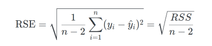
Degrees of freedom

Accounts for each parameter, variance estimate become unbiased

• n-p-1

Total Sum of Squares

Total variability in the response

R²

Proportion of variability accounted for in the model

F-statistic

tests whether the model as a whole is useful: is there any real relationship between the predictors and the response, or could the whole thing be noise?

• Above 1

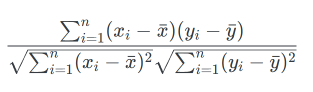
Correlation coefficient

Measures linear association between two variables

• Simple: R²=r²

Assumption: Linearity

the relationship between the predictor and the response is linear

• a residual plot, should show no curvature

Assumption: Errors Do Not Track the Predictors

After accounting for the predictors in the model, the leftover errors should not systematically rise or fall with those predictors

Omitted variable bias

Variables correlated with the X or Y that is not outlined in the model can sit in the error, making the X look better or worse

Independence of Errors/Autocorrelation

Each observation’s error is independent of the others (fails in time series and clustered/duplicated data); lowers standard errors

Constant Variance / Homoskedasticity

Each observation’s error is independent of the others X

• the residual plot should look like random scatter with equal spread everywhere, no funnel shapes

Normality of errors

The errors ε follows a normal distribution

• a histogram of the residuals should look roughly bell shaped and centered at zero, and a Q-Q plot of the residuals should follow a straight line

exact t and F distributions for inference in small samples

Assumptions: Linearity & Independence of Errors

the least squares coefficients are unbiased: on average across repeated samples, they land on the truth

Assumptions: Linearity & Independence of Errors & Independence & Constant Variance

The Gauss-Markov result: among all linear unbiased estimators, least squares has the smallest variance

Breusch-Pagan Test

The null hypothesis: the errors have constant variance (homoskedasticity)

The alternative: the error variance changes with the predictor(s) (heteroskedasticity).

Leverage

Point with potential to pull line towards itself

Cook’s distance

measures how much the fitted model would change if we deleted each observation

• Flagged above 1

Parsimony

the simplest model that does the job

• Some predictors are costly or unreliable to collect. If newspaper data requires a paid subscription and contributes nothing, drop it.

• Smaller models are easier to interpret and explain to stakeholders.

• Unnecessary predictors add noise and can hurt predictions on new data.

• Fewer predictors mean fewer missing value headaches and less multicollinearity.

forward selection

start with nothing, add the most useful predictor one at a time

backward elimination

start with everything, remove the least useful one at a time

stepwise selection

a hybrid that can add and remove

Data amount: Signal strength

Large effects are easier to detect regardless of sample size

Data amount: Noise

A high residual variance demands more data for the same precision

Data amount: Collinearity

Correlated predictors inflate standard errors, and heavily overlapping predictors can burn through a sample fast

Data amount: Prediction vs. Inference

Stable prediction and precise inference about a specific coefficient have different appetites

Adjusted R-squared

Adjusted R² will not necessarily go up when adding new predictors

Test Mean Absolute Error (MAE)

It is in the same units but weights every miss equally instead of punishing large ones, so a big gap between RMSE and MAE tells you the errors are dominated by a few bad misses

Collinearity

Correlation among predictors that destabilizes coefficient estimates

Variance Inflation Factor

Quantifies how much collinearity inflates the variance of each coefficient

• Problem: above 5 or 10

Qualitative predictors

represent discrete groups or categories

• Ordinal: ordered

• Nominal: unordered

dichotomous

two level

polytomous

3 or more levels

dummy variables

converts a categorical predictor with k levels into k−1 dummy variables, each taking the value 1 or 0.

baseline

category absorbed into the intercept

No significant intercept

• If the baseline value is something you need to interpret or report, look into why it is imprecise.

• If you are focused on prediction, the intercept is just part of the machinery; overall accuracy is what matters.

• If predictors can never realistically be zero (a GNP of $0 means civilization has ended), the intercept is a mathematical anchor, not a meaningful quantity, and its p-value is a non-issue

Dummy Intercept interpretation

the average units of the baseline

Dummy Slope Interpretation

X units in compared to the baseline

Interaction

when the effect of one predictor on the response depends on the value of another predictor

Interpretation: Interaction Coefficient

measures how much the effect of X1 changes per unit increase in X2

how much the X1 slope grows/slows with each additional unit of X2

β 1 is the effect of X1 when X2=0: the baseline slope

The Hierarchical Principle

Keep main effects, even if not significant, when including and interaction term

Centering coefficients

Subtract means from values

Intercept: predicted Y at average Xs

Slope: predicted effect of X1 at average X2

Helps with multicollinearity

Dummy and Interaction

the dummy moves intercepts, the interaction moves slopes

Additive assumption

the effect of each predictor is the same no matter what the other predictors are doing