3.3 Revenue, Costs and Profits

Business objectives

Profit maximisation

Revenue maximisation

Sales maximisation

Profit maximisation

When a firm tries to generate the highest possible total profit from the production of a good/service (maximise the difference between total revenue and total costs)

Occurs when marginal revenue is equal to marginal cost

Profit maximisation diagram

When MR>MC, profits↑

When MR<MC, profits↓

Revenue maximisation

When a firm tries to generate the highest possible total revenue from the production of a good/service (maximise total revenue)

Occurs when marginal revenue is 0

Revenue maximisation diagram

When MR>0, TR↑

When MR<0, TR↓

Sales maximisation

When a firm tries to generate the highest possible sales from the production of a good/service, without making a loss

Occurs when average revenue is equal to average costs

Sales maximisation diagram

P>AC, a loss is not made

P<AC, a loss is made due to too many sales

Business objective diagram

Q₁ and P₁ is the quantity and price where a firm maximises profit

Q₂ and P₂ is the quantity and price where a firm maximises revenue

Q₃ and P₃ is the quantity and price where a firm maximises sales

Profit maximising inherently reduces sales, and sales maximising inherently reduces profit

Revenue maximising is the best of both worlds

Revenue

Revenue refers to the monetary income earned by a firm from selling a good/service over a given period of time

Total revenue

Total revenue refers to the monetary income earned by a firm from selling all units

Average revenue

Average revenue refers to the monetary income earned by a firm per unit sold

Marginal revenue

Marginal revenue refers to the monetary income earned by a firm from the last unit sold

Explaining the shape of the average revenue curve

The average revenue curve models the demand curve of a firm as at any given quantity, average revenue is equal to the price (can be derived from its formula); thus, a curve that plots price against quantity (i.e. the demand curve) will be the same as one that plots average revenue against quantity (i.e. the average revenue curve)

Explaining the intercepts of the total revenue curve

When the quantity is 0, there are no customers and hence no revenue

When the price is 0, no money is charged and hence no revenue

These both can be derived from the formula total revenue = price x quantity (when either is 0, total revenue is 0)

Explaining the shape of the total revenue curve

When marginal revenue is greater than 0, total revenue is rising, meaning money was made on the last unit sold

When marginal revenue is less than 0, total revenue is falling, meaning money was lost on the last unit sold

As marginal revenue gets smaller (but still greater than 0), the increase in total revenue gets smaller; as marginal revenue gets even smaller (less than 0), the decrease in total revenue gets larger

Explaining the steepness of marginal revenue

AR = -mQ + c

TR = PQ, where P = -mQ + c

TR = -mQ² +Qc

MR, which is the derivative of TR, = -2mQ + c

Therefore, MR’s gradient is two times the gradient of AR

Explaining the relationship between PeD and total revenue

Between A and B, prices are falling, quantity is rising, and total revenue is rising; therefore, PeD must be elastic

Between B and C, prices are falling, quantity is rising, and total revenue is falling; therefore, PeD must be inelastic

At point B, PeD is unitary; hence, PeD is 1

Short-run production theory

In the theory of the firm, the short run is defined as any period of time in which a firm is unable to increase all factors of production; i.e. at least one factor of production is fixed

The problem with short-run production theory

The law of diminishing marginal returns refers to the decrease in the additional output generated from adding the last variable factor of production

Firms will always face the law of diminishing marginal returns if they expand output in the short run, as eventually they will end up overspecialised in one factor of production

Marginal product/output diagram

Law of diminishing marginal returns occurs at point A

Marginal cost

Marginal cost refers to the cost of the factor resources necessary to produce the last unit

MC = Δ total costs / Δ quantity

Explaining the shape of the marginal cost curve

The shape of the marginal cost curve can be explained by the law of diminishing marginal returns; initially, as variable factors of production are added to the fixed factor, productivity increases, so firms pay less for the extra output, so marginal cost falls (A to B)

However, eventually diminishing marginal returns occur as production becomes over-specialised in the variable factor; as productivity falls, firms are paying more for each extra output, so marginal cost rises (B to C)

Average costs

Average costs refer to the cost of factor resources necessary to produce on a per-unit basis, over a given period of time

Total costs

Total costs refer to the cost of factor resources necessary to produce all units, over a given period of time

Fixed costs

Fixed costs do not change with output

(e.g. rent)

Variable costs

Variable costs change with output

(e.g. wages, energy and raw materials)

Total costs formula

Total costs = total fixed costs + total variable costs

Total costs = average costs x quantity

Average costs formula

Average costs = average fixed costs + average variable costs

Average costs = total costs / quantity

Total fixed costs diagram

Total fixed costs do not change with output (at any given quantity, cost is always C₁)

Total variable costs diagram

Total variable cost is the integral of marginal cost

Total variable cost always starts at the origin, as with no output, there are no variable costs

As the last units get cheaper, total variable costs increase by less; however, as the law of diminishing marginal returns sets in and the last unit becomes more expensive, total variable costs increase at a faster rate

Total cost functions diagram

The vertical distance from total costs to total variable costs is C₁ (which is the total fixed costs)

Total costs have the same gradient/shape as total variable costs and starts at C₁

Average fixed costs

Average fixed costs diagram

Average fixed cost curve slopes downward as total fixed costs are spread across more units

Average variable costs

Average variable costs diagram

If the marginal cost is below the average variable cost, the average cost is pulled down; as soon as the marginal cost overtakes the average variable cost, it pulls it up

If MC<AVC, AVC↓

If MC>AVC, AVC↑

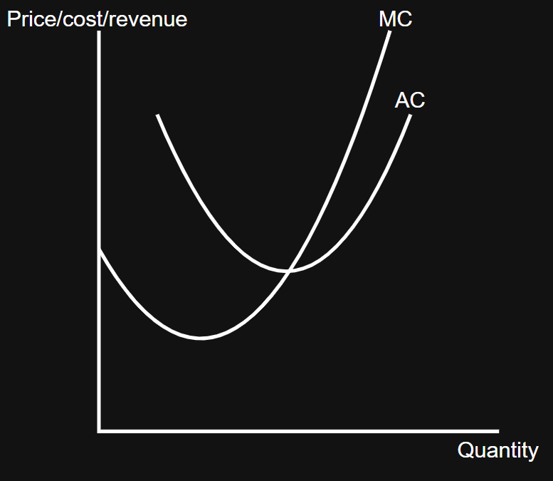
Average costs functions diagram

The gap between average cost and average variable cost gets smaller with output as less is being added to average variable cost (because the average fixed cost is decreasing)

Full model of the firm

Total functions are not used as TR = AR x Q and TC = AC x Q, with Q being on the x-axis; therefore, the area under a point on AC or AR gives you the TC or TR, respectively

Variable and fixed costs are excluded from the basic model, as profit can be calculated from just TC; however, some advanced models do require distinction between fixed and variable (e.g. shut-down point models)

Economies of scale

The cost advantages a firm gains as its scale of output rises in the long run, which lowers the long-run average cost (LRAC)

Types of economies of scale

Internal economies of scale

External economies of scale

Internal economies of scale

Occurs when a firm increases the scale of production within the firm (e.g. technical, purchasing, financial, research and marketing)

Movement along the LRAC curve

Occurs due to a change in the internal economies/diseconomies of scale of a firm

Internal economies of scale - technical

Large businesses can afford specialist machinery that small businesses cannot, helping them to produce more cheaply

The productivity of capital increases where output rises faster than total costs, reducing average costs and the unit cost of production

Internal economies of scale - purchasing

Large firms can buy raw materials in bulk, allowing them to negotiate a large discount per unit; this means that total costs will be rising, but at a slower rate than output, reducing the average cost of production

Large firms can do this if they have monopsony power

Large firms have huge warehouses to store goods in, something small businesses cannot benefit from

Internal economies of scale - financial

Large firms are safer to lend to, and hence banks may negotiate lower interest rates on loans for investment projects

Larger firms will also be borrowing larger sums of money, which does not significantly increase the marginal costs for banks, thus keeping interest rates low

Total costs are rising, but more slowly than output, reducing the unit cost of production

Smaller firms usually have to go to high street banks or raise capital from friends or family

Internal economies of scale - marketing

Advertising costs can be spread across many stores

Adverts can be bulk-bought to help negotiate a lower price with TV channels and newspapers

Large businesses can employ specialist staff

Internal economies of scale - research

Lower enterprises can allocate more resources to research and development of new products or processes

Internal economies of scale - risk-bearing

Large firms can afford to take risks with new goods/services because other parts of the business are still profitable

External economies of scale

Occurs outside of the firm and within an industry, all competitors benefit (e.g. labour-market pooling, agglomeration economies and research spill overs)

Shift in the LRAC curve

Occurs due to a change in external economies/diseconomies of scale of a firm

External economies of scale - labour-market pooling

Firms in the same industry share access to a large pool of specialised workers; workers also benefit because they have many potential employers nearby

This creates a two-way effect; firms attract skilled workers, and skilled workers attract more firms

External economies of scale - agglomeration economies

When many firms locate close together, they can experience lower costs and higher productivity because infrastructure, suppliers, services, information, and customers become concentrated in one area

External economies of scale - research spill overs

Knowledge created by one firm can benefit other nearby firms, with ideas being spread through worker movement, universities, suppliers, networking and observation

Therefore, firms can innovate faster without paying fully for research and development, raising productivity and reducing average costs

Diseconomies of scale

A rise in the long-run average costs of a firm as output rises

Types of diseconomies of scale

Internal diseconomies of scale

External diseconomies of scale

Internal diseconomies of scale

When a firm’s long-run average cost per unit increases as a result of the company growing too large

Internal diseconomies of scale - communication

There may be barriers to communication in larger organisations, which could lower morale and productivity

Internal diseconomies of scale - control

Large firms may become difficult to manage and require more layers of bureaucracy

Internal diseconomies of scale - coordination

Costs of administration and coordination of the workforce in different time zones and languages

External diseconomies of scale

When a firm’s long-run average cost per unit increases as a result of outside factors affecting the industry

External diseconomies of scale - input-price inflation

This happens when lots of firms cluster in the same area and compete for the same scarce inputs, such as land, office space, electricity, transport, or raw materials

External diseconomies of scale - wage-bidding

When many firms in the same area need workers with similar skills, they compete against one another to hire them

Minimum efficient scale

The output for a firm in the long run, where the internal economies of scale have been fully exploited

It corresponds to the lowest point on the long run average total cost curve

Minimum efficient scale in different industries

The size of the MES differs across industries based on technology, setup costs, and total market demand

High minimum efficient scale industries

Sectors which require massive upfront capital and high fixed costs; unit costs drop significantly only when output is extremely high

As the MES is a large percentage of the total market demand, these markets are often natural monopolies or oligopolies

(e.g. utility and automotive industries)

Low minimum efficient scale industries

Sectors which require little initial investment, meaning barriers to entry are low, resulting in a fragmented market structure filled with many small, independent firms competing locally

Firms in these industries reach their lowest cost per unit at low levels of output

(e.g. local restaurants or hair salons)

Profit maximisation

Within the cost/revenue model, all firms achieve maximum profits at the output level where MR=MC

When MR>MC, the last unit is profitable, meaning total profits are rising

When MR<MC, the last unit makes a loss, meaning total profits are falling

This means that where MC=MR, the firm has produced all the units that increase profits, but none of the units that decrease profits

Normal profits

Occurs when a firm’s revenue covers the actual cost and opportunity cost of production (AR=AC); i.e. the profit that could be made elsewhere

At normal profit, firms will neither enter nor leave the industry

Supernormal profits

Occurs when a firm’s revenue exceeds the actual cost and opportunity cost of production (AR>AC); i.e. more profits are made than could be made elsewhere at supernormal profits, hence new firms will attempt to enter the industry

Losses

Occurs when a firm’s revenue does not cover the actual cost and opportunity cost of production; i.e. less profitable than could be made elsewhere (this always includes breaking even); at this level of profit, incumbent firms (pre-existing firms in the market) will leave the market

Profit diagram

AR>AC - supernormal profit

AR = AC - normal profit

AR<AC - losses

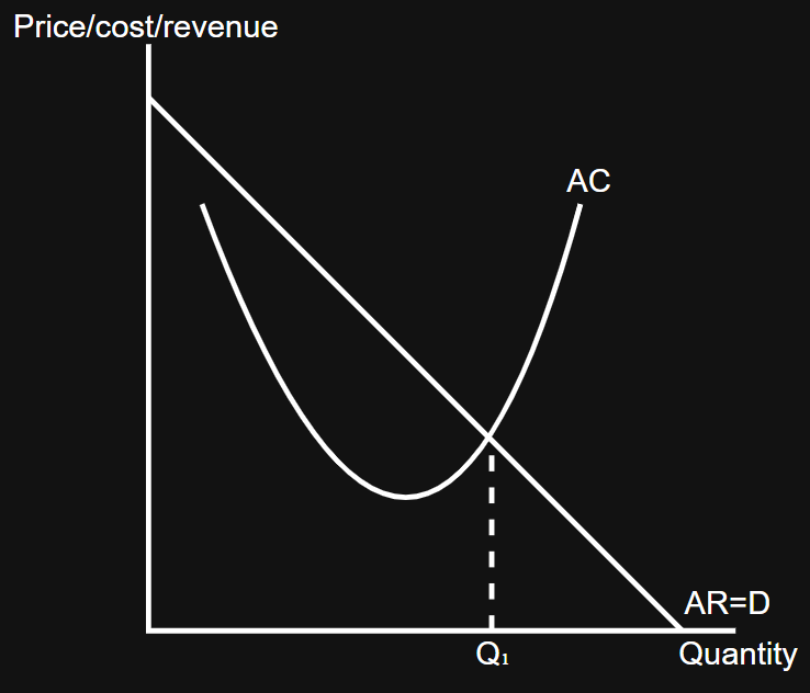
Optimum profit diagram

Q₁ is the optimum output for profit, and P₁ is the price to sell at for optimum profit

Area X represents the profit made from selling at that price and quantity; the area for profit can also be represented by the formula Q₁ x (P₁ - C₁)

Area Y represents the costs incurred from selling at that price and quantity

Price maker in all profit/loss states - profit

AC is below AR

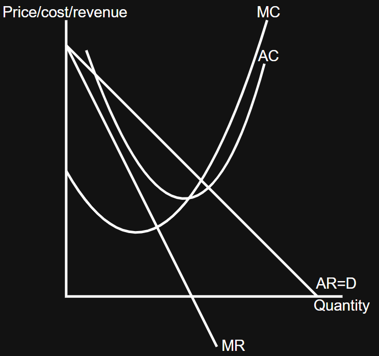
Price maker in all profit/loss states - loss

AC is above AR

Price maker in all profit/loss states - profit maximising with normal profit

AR is equal to AC at Q₁

Shut-down points

Concerns whether firms should or should not leave the market when making a loss

Short-run shut-down points

If a firm makes losses in the short run, it may not necessarily shut down immediately

Occurs when P≥AVC

Short-run shut-down points diagram

If P≥AVC, the firm can cover all of its variable costs with revenue and also pay off all of its fixed costs

Long-run shut-down points

If a firm makes losses (TC>TR), it will always leave the market/shut-down in the long run

Occurs when P<AVC

Long-run shut-down points diagram

If P<AVC, the firm is unable to cover all of its variable costs with revenue; hence, to minimise loss, it should leave the market immediately

Evaluation for shut-down points

Use the short-run shutdown points theory as an evaluation; i.e. even though a firm is making a loss, it should not have to shut down immediately if P≥AVC

If a firm can find a way/excepts future revenue to rise/fall, it might not have needed to shut down (if it can sustain losses with savings/investor capital)

In recent history, many large publicly traded firms have sustained losses without needing to shut down, e.g. Uber; if firms can operate for many years without making losses, losses by themselves do not explain or guarantee a shutdown