STAT200

Frequency Table

Shows all the categories of a categorical variable with their frequencies (as a %)

% add up to 100

Contingency Tables

Between 2 categorical tables

Row and column totals, grand total

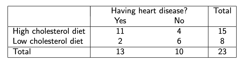
Simpson’s Paradox

when a third variable changes the relationship between 2 categorical variables

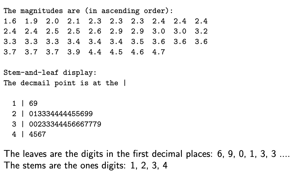
Stem-and-lead display

Stem - 1+ leading digits, vertical column

Lead - 1 trailing digit, horizontal, no repeats

Use only for small data ses

Describing distribution of quantitative data

1. Shape

• Unimodal/bimodal/multimodal (# of peaks)

• Skewed (right - right hand tail, left - left hand tail)

• outliers

2. Center (median or median)

• Median:

  • Odd = (n+1)/2, where n = number of observations

  • Even = average of n/2 and n/2 +1

3. Spread

• Range

• IQR

• Variance/Sd

  • Variance: sum of the squared values of (observation-mean)/(n-1)

  • Sd: variance ²

  • Will always be non negative

  • If = 0, observations are all equal

Plotting outliers on boxplots

Fall above Q3 + 1.5*IQR or below Q1 - 1.5*IQR

Whiskers extend to the smallest and largest observations not flagged as outliers

Sensitivity to outliers

Sensitive: mean, range, variance, SD

Not sensitive: median, IQR

When to use which summary statistic

If the distribution is roughly symmetric: mean/variance/SD

Skewed distribution: median/IQR

Hows does shifting data affect mean, SD, and other summary statistics

Shifting: add a constant, c, to each observation

Median/Mean: shifted by c

Variance/SD/Range/IQR: does not change spread

Hows does scaling data affect mean, SD, and other summary statistics

Scaling: multiply each observation by positive constant, c

Both centre and spread will change and be multiplied by constant c

Variance will be c² times the original variance

Standardizing

z-score = deviation from mean/SD = observation - mean/SD

Meaning:

• + = observation has a value below the mean

• z = k = observation that is k many SD above the mean

• z = -k = observation is k many SD below the mean

• the further the z score is from 0, the further the observation is from the mean

• z = 0 means the observation = mean

Normal model

• bell-shaped, unimodal

• perfect symmetry around the mean μ

• Spread is determined by SD σ

• Model is denoted by N (μ, σ) → N (0,1)

• mean and SD are parameters (numerical characteristics of a model)

• Follows 68-95-99.7 rule

Standardizing values from the normal model

z = observation - mean / SD

Mean = 0

SD = 1

Scatter plots

between 2 quantitative variables

mean-mean point (x̄, ȳ) provides the center of the cloud of data

points

Types of patterns of a scatterplot

1. direction

2. form: linear/non-linear

3. Strength of relationship

• Use correlation coefficient to measure strength of linear relationship

4. outliers

Properties of correlation coefficient r

between -1 and 1, no units

r close to 0 implies weak or no linear relationship

swapping x and y variables does not affect r

value does not change if a constant is added/multiplies to observations

sensitive to outliers

DOES NOT = SLOPE

Formula: sum of products of standardizes x and y values /( # of observations - 1)

Regression line

slope r* SD(y)/SD(x)

r = correlation coefficient, SD(y)/SD(x) standard deviation of x and y data

Intercept = ȳ - (slope)*x̄

line passes through mean-mean point (x̄, ȳ)

Model relating x and y is ŷ = mx+b

ŷ = predicted value

Residuals

The difference between the observed value and the predicted value from the residual line

e = y - ŷ

• sum of residuals always = 0

• make a residual plot to assess the appropriateness of the regression model

  • if the model is appropriate, the residual plot will show no pattern

Influential points

data points whose omission results in a very different fitten regression model

Lurking variables

a variable that is the underlying cause for an association between 2 variables

Things to watch out for when fitting a linear model

1. x and y have to have a sufficiently linear relationship

2. do not extrapolate (prediction about y for values of x that lie outside the observed range the linear model is built in)

3. outliers highly influence the model

Why do we have randomization

to obtain a representative sample

Sampling Methods - Simple random sampling

N individuals sampled at random from the population

Sampling Methods - Stratified Sampling

Divide population into a strata based on a particular characteristic

Simple random sample drawn from each stratum

smaller variability across samples → more reliable results

Sampling Methods - Cluster Sampling

With natural groupings in the population

Simple random sampling of clusters

2 stage cluster sampling: a simple random sample is drawn from samples in selected clusters

Sampling Methods - Multistage sampling

1+ stage or sampling procedure (2-stage cluster)

Sampling Methods - Systemic Sampling

selecting every kth individual from the sampling frame

sampling frame should not contain any hidden order

Bad sampling procedures

1. undercoverage: excludes/underrepresents certain kinds of individuals

2. convenience sampling: selection of individuals based on easily availability

3. voluntary response bias: for voluntary surveys, individuals with strong opinions will respond more often

4. nonresponse bias: individuals who dont respond to surveys

5. response bias: response is influenced by how the question is asked or misunderstanding of the question or lies

Observational Studies

examining the association between 2 variables

no human intervention

retrospective vs prospective study

prospective studies: individuals are followed over time and data about them is collected as their characteristics or circumstances change retrospective studies:individuals are sampled and information is collected about their past

Experiments

planned intervention on the exposure to a condition suspected of altering a response outcome

cause and effect relationship can be established

randomized comparative experiments

Assess the effect of an explanatory variable, factor, on a response variable

Compare the response variable between different levels of a factor

Control the type of treatment individuals receive

Principles of experimental design

1. randomize

2. replicate

3. blocking: control variables that are not factors but can influence the response, improving accuracy of comparison (ex. male and female groups)

Blinding

Single-blind: either experimental units or evaluators are blinded to the treatment assignment

Double-blind: both experimental units and evaluators are blinded

Types of experiments

1. completely randomized: treatments are randomly assigned, no blocking

2. Randomized block: subjects are separated into blocks, treatment assignment is done within separate blocks

3. matches pairs design: subjects are matched in pairs by characteristics that may affect response

Lurking variable vs confounding variable

lurking: effects both variables, results in an apparent relationship between variables even though there’s no causation between then

Confounding: associates with both variables but you cannot distinguish between the effect of the confounding variable on the response or the effect of the explanatory on the response

Sample space

S, set of all possible outcomes of a random phenomenon

{x,y,z,…}

Probability of an event

0 < P(A) < 1

0 = impossible, 1 = certain

sum of probabilities of all non-overlapping events = 1

How to tell if two events are independent

occurrence of A does not alter the probability that B will occur, and the other way around

P(A|B) = P(A) → probability of A given B = probability of A

P(B|A) = P(B)

Probability that A and B will occur together:

P(A∩B) = P(A) * P(B)

Conditional Probability

Probability of A given B = Probability of A and B/Probability B

P(A|B) = P(A∩B)/P(B)

and

Probability of A or B:

P(A∪B) = P(A) + P(B) - P(A∩B) 

Discrete random variables

possible values are either a finite set or an infinite sequence of values

continuous random variable

possible values are in an interval on the number line or all numbers in a collection of intervals

described with density curved: denoted by f(x)

probability that continuous random variable X takes on a value

between a and b is the area under the density curve over (a, b):

• total area under density curve = 1

uniform random variables

density curve is a straight line (area under the curve is a rectangle/square)

Mean:(a+b)/2

Standard deviation: √((b-a)²/12)

mean + variance of random variables

mean: long-run average of the values taken on by the random variable

• tells where the centre of the distribution lies

variance + sd: measures how spread out values taken on by the random variable are

Binomial Experiments

1. Consists of n identical trials. The number of trials is fixed in advance. 

2. The outcomes on each trial can be dichotomized into two complementary categories: “success” and “failure”. 

3. The probability of the success event, p, is the same from trial to trial. The probability of the failure event is q = 1 − p. 

4. The n trials are independent of each other. In other words, the results of previous trials do not affect the result of the current trial.  

Mean, variance and standard deviation of the binomial random variable

Mean: np

• average # of successes if you are to repeat the experiment many times

Variance: np(1-p)

• variability of the # of success if the experiment is repeated many times

SD: √variance

Bernoulli random variable

A random variable that takes value 1(Success) and 0 (Failure) 

Bernoulli trials has only two possible outcomes. One is called Success and the other one is called Failure. 

• X(Success) = 1 

• X(Failure) = 0 

where 

• P (Success) = p 

• P (Failure) = 1 − p 

Population

The entire collection of individuals

Sample

A subset of individuals selected from a population

Parameter

Numerical summary of a population

fixed and unknown

Statistic

A random variable used to estimate population parameters

Sampling distribution of proportions (percentages)

true proportion of individuals sharing a certain characteristic in a population is : 0<p<1 (parameter)

For a sample of n individuals randomly selected, the sample proportion (statistic) is:

p̂ = # of individuals samples who have the characteristic/n

• used to estimate the true population proportion

• varies across samples and doesnt equal p

sampling distribution of p̂

distribution of the sample proportions of all random samples of size n that can be obtained from a population

Mean → µ(p̂) = p

For large samples, the sampling distribution of p̂ is approximately Normal

• larger the n = better the normal approximation

• N(mean,variane)

Assumptions and conditions for the validity of normal approximation

1. sample is randomly drawn

2. individual values in the sample are independent

3. the same size is large

• np ≥ 10

• n(1-p) ≥10

sampling distribution of means

The population mean μ is a parameter, which is fixed but usually unknown. The sample mean ȳ is a statistic and is used to estimate the true population mean μ. 

sample mean of a measurement: ȳ = total of y values/n

The sampling distribution of means is the distribution of the means of all the possible random samples of size n that could be selected from a population. 

• The mean of the sampling distribution of means is denoted by μ(ȳ), and is equal to μ in value. 

• The standard deviation of the sampling distribution of means is denoted by σ(ȳ). Its value is given by σ(y) = 𝜎/√n 

The Central Limit Theorem (CLT)

• For sufficiently large samples, the sample mean y follows approximately the Normal model, even if the underlying distribution of the individual observations in the population is not Normal. 

  • always hold true regardless of the sample size n. 

• The larger n = the smaller the sd for the sample means, and the better the approximation of the Normal model to the sampling distribution of y

a) Model is appropriate. b) Model is not appropriate. Relationship is nonlinear. c) Model may not be appropriate. Spread is changing.

a) 1)  High leverage, small residual. 2) No, not influential for the slope. 3)  Correlation would decrease because outlier has large zx and zy, increasing correlation. 4)  Slope wouldn’t change much because outlier is in line with other points.

b) 1) High leverage, probably small residual. 2) Yes, influential. 3)  Correlation would weaken, increasing toward zero. 4)  Slope would increase toward 0, since outlier makes it negative.

c) 1) Some leverage, large residual. 2) Yes, somewhat influential. 3) Correlation would increase, since scatter would decrease. 4) Slope would increase slightly

d) 1) Little leverage, large residual. 2) No, not influential. 3)  Correlation would become stronger and become more negative because scatter would decrease. 4) Slope would change very little.