Macro lec 6

equilibrium in the IS LM model

The intersection determines the unique combination of Y and r that satisfies equilibrium in both markets. 

Because the interest rate influences both investment and money demand, it is the variable that links the two halves of the IS–LM model. 

The model shows how interactions between the goods and money markets determine the position and slope of the aggregate demand curve and, therefore, national income in the short run.

inc in government purchases

An increase in government purchases increases planned expenditure, resulting in increased  

production and income, represented by the shift of the IS curve to the right. 

• The equilibrium moves from point A to point B. Income rises (i.e. fluctuates) from Y₁to Y₂, and the interest rate rises from r₁to r₂.

The economy starts in equilibrium where the goods market (the IS curve) and the money market (the LM curve) are both in equilibrium, at a unique combination of r and Y. Suppose the government wants to raise income and increases its purchases. This raises planned expenditure and shifts the IS curve to the right by ΔG/(1 − MPC) (or 1/(1 − MPC) x ΔG) , the size of the government purchases multiplier effect. Higher income affects not only the goods market, through the multiplier process, but also the money market, because higher income means more transactions and therefore a higher demand for money. According to the theory of liquidity preference, which the LM curve is derived from, a higher demand for money with a fixed money supply pushes up the interest rate. The economy therefore moves up along the unchanged LM curve. The higher interest rate feeds back into the goods market and lowers investment. This is crowding out. As a result, in the short run, the final increase in income is smaller than the multiplier effect ΔG/(1 − MPC) would suggest.

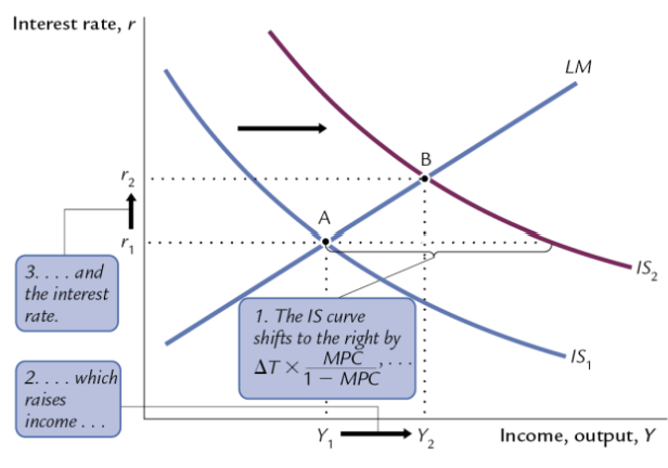
a tax cut

When you decrease taxes it increases planned expenditure which pushes the IS curve to the right, it shifts the IS curve by the amount as indicated by the tax multiplier, meaning that at every interest rate income would increase by change in the tax multiplied by the government purchases multiplier. ΔT × MPC × 1/(1 − MPC), where MPC × ΔT is the first-round change in spending and 1/(1 − MPC) is the usual spending multiplier. This is why the tax multiplier is smaller than the government spending multiplier. The additional income moves along the LM curve as income increases it pushes up money demand  and the interest rate increases, because the interest rate is increasing and investment starts to go down and there's this crowding out again so that the final increase in income is not as large as indicated by the government tax multiplier 

an increase in the money supply

 An increase in the money supply shifts the LM curve downward. 

An increase in the money supply (with prices fixed) raises real money balances, which creates an excess supply of money at the current interest rate. People put the extra money into bonds or deposits, and banks and bond issuers respond by offering lower interest rates. The interest rate falls until people are willing to hold the larger money stock, which restores money market equilibrium.

The lower interest rate raises investment demand, which raises output and income through the multiplier. The higher income raises money demand, which pushes the interest rate back up a little, but not all the way back to where it started. So the final fall in the interest rate is smaller than the initial fall.

In IS-LM terms, expansionary monetary policy shifts the LM curve out (right/down), and the economy moves down along IS. The result is a lower interest rate and higher GDP. The chain from the money supply to GDP (higher M → lower r → higher I → higher Y) is called the monetary transmission mechanism.

The Monetary Policymaker’s response to ΔG > 0

Response 1: Hold M constant 

• An increase in G shifts the IS curve out. The central bank holds the money supply constant, and therefore, the LM curve stays the same. Both income and the interest rate rise.

Response 2: Hold r constant 

• An increase in G shifts the IS curve out.  

• To keep r constant, the central bank then increases the money supply. 

• Income increases by more than if the central bank held M constant.

Response 3: Hold Y constant 

• An increase in G shifts the IS curve out.  

• To keep Y constant, the central bank then decreases the money supply.

The Monetary Policymaker’s response to  Increase in Taxes (contractionary)

• Suppose the fiscal authorities increase taxes. 

• Other things being equal, this would reduce output and interest rates in the short run.  

• If the central bank was trying to keep interest rates stable, however, it would respond to this change by decreasing the money supply. The result would be a larger decrease in output. 

• Alternatively, the central bank might be trying to keep output stable, in  which case it would increase the money supply, driving interest rates down further.  

• The basic lesson is that the ultimate effects on the economy depend  upon the combinations of policies chosen by the monetary and fiscal  authorities.

• Lower income means lower demand which means that the interest rates would fall

IS shocks

• IS shocks: exogenous changes in the demand for goods and  services 

• For example, the “animal spirits” of business people shift the IS  curve.  

• Similarly, changes in consumer confidence alter consumption  behavior and cause the IS curve to shift.  

• Any change in business or consumer confidence or expectations  shifts the IS curve

LM shifts

• LM shocks: exogenous changes in the demand for money 

• For example: 

• During Covid-19, consumers and companies did not wish to handle  cash and switched to more cashless methods of payments. 

• More ATMs or the internet reduce money demand.

From the IS–LM Model to the Aggregate Demand Curve 

Aggregate demand summarizes equilibrium in both of these markets. 

• Recall that the IS–LM model is constructed on the basis of a fixed price level.

 Any change in the real supply of money shifts the LM curve. The real money supply changes if either the nominal money supply or  the price level changes. Thus, we can see that changes in the price  level are associated with changes in the equilibrium level of GDP  and interest rates in the IS-LM model. This is the relationship that is  summarized by the aggregate demand curve.

price level and the money supply

• If the price level is high, other things being equal, the real money supply is low. This implies high interest rates and thus low investment and output.  

• If the price level falls, then the real money supply increases.  Equilibrium in the money market implies that interest rates must  fall. Equilibrium in the goods market thus implies that GDP must  rise, since investment rises.  

 Thus we find that the aggregate demand curve is downward  sloping; high values of the price level are associated with low  levels of GDP and vice versa. 

Monetary policy and the AD curve 

 ↑M → LM shifts right, → ↓r,→ ↑I, → ↑Y at each value of P.

Fiscal policy and the AD curve 

 Expansionary fiscal policy (↑G and/or ↓T) increases  aggregate demand: ↑G,→ IS shifts right,→ ↑Y at  each value of P

how does the economy move from short run to long run

The force that moves the economy from the short run to the long  run is the gradual adjustment of prices. 

the difference between a movement along the Aggregate Demand (AD) curve and a shift of the entire AD curve

1. Movement along the AD curve – Change in price level

When the price level changes, this causes a change in income/output (Y) within the IS–LM model. This represents a movement along the existing AD curve because the price level itself is one of the variables represented on the AD graph.

2. Shift of the AD curve – Change in income at a given price level

When something other than the price level changes income/output (Y), the entire AD curve shifts. This happens because income changes even though the price level remains constant.

the spending hypothesis

• The IS–LM model teaches that an inward shift in the IS curve  reduces income and interest rates. Since nominal interest rates  fell during the Depression, negative shocks to the IS curve are one  possible explanation. This is the spending hypothesis.  

the money hypothesis

A monetary contraction shows up in the IS–LM model as an inward  shift of the LM curve, which would reduce output.  

• There are two problems with this money hypothesis, however. The  first is that prices also fell substantially over this period, so real  money balances actually increased slightly between 1929 and  1931, although they did fall between 1931 and 1933. The second  problem is that an inward shift of the LM curve should be  associated with rising interest rates

why AD curve is negatively sloped

 negative slope because ↑P → ↓(M/P) → ↑r → ↓I → ↓Y