PsychStats 240: Exam 1

stats branches

descriptive and inferential

population

the group youre studying

sample

the group of people you take from the pop.

how to get a random sample

you can # everyone and randomly generate a group

sample of convenience

members of a pop. that you easily have access to as long as it’s representative of the pop.

descriptive stats vs inferential stats

summarizing data vs drawing inferences from the pop.

continuous vs discrete numerical/quantitative variables

Continuous: any #, can be decimals (ex: weight)

Discrete: only whole #s (ex: number of siblings you have)

Ordinal Scale

-order of valuess - he variables are in order, the differences between them have no intrinsic meaning (ex: a self reporting scale a satisfaction from 1-5, two people rating their sat. a 4 might have different interpretations of what that means)

Interval scale

- interval between values- ordered and equal intervals, no true 0 (ex: temperature, 0F/C does not mean there is an absence of temp)

Ratio scale

-ratio of values- t has a true 0! (ex: money, you can have no money) the ratio between quantities is interpretable, you can have 2x as much $$ but not 2x as much temp or IQ

contingency table

a two-way table that shows the distribution of two categorical V

why aren’t pie charts helpful?

they just show the % instead of actual amount

histogram

no space between bars, if it looks like your right foot it’s right skewed

one hump: unimodal

two: bimodal

none: uniform/rectangle

mean formula:

x(w bar=mean) = x1+x2+…../xn OR mean=1/nExi (the sum of all x’s divided by the number)

variance

the spread of variables around the mean

S2= (x1-mean)2+…./n-1 or S2= 1/n-1E(xi-mean)2

squaring makes it positive

SD

average distance of a variable from the mean

skews influence:

the mean, but not the median

IQR

range from Q1 to Q3

Whiskers

extend to max and min unless there are values more than 1.5x the IQR

boxplots are helpful for

comparing 2+ distributions

dominant view/frequentist view

the prob of a probability occuring exactly only happens over a large amount of trails (ex: flipping a coin heads 50% of the time would take hundreds of flips)

probability

cant be less than 0 or greater than 1, the sum of the prob of various possible events that can happen must =1

probability distribution

instead of logging the actual time each value occurs, you log the probability of it occurring

discrete distributions

the outcomes are defineable and have a limited number of possibilities ex( the # of jean types i can wear- theres only so many)

continuous distributions

no 1 value of this variable will have any probability assigned to it, instead we assign the gap between two probs ex( the probability of women between 5’1 and 5’2)

Continous distributions use what graph/function

PDF probability density function - density curve

Measures the gaps between two values

the area underneath is 1, the y’s must adjust to the x’s to make the area 1.

Binomial distributions

probability of the # of times an event happens in n trials, if the event has a fixed probability on each trial (that’s why they’re often ALMOST normal distributions)

ex: coin flips: p(heads)=.5, n+100

a success in stats is

when what were studying happens (ex: flipping heads)

how to get the probability of smth with multiplication

if p(make)=.7 and you want to know the prob of making 8/10 shots multiply

.7 (8times) + .3 (2 times)

Normal Distribution

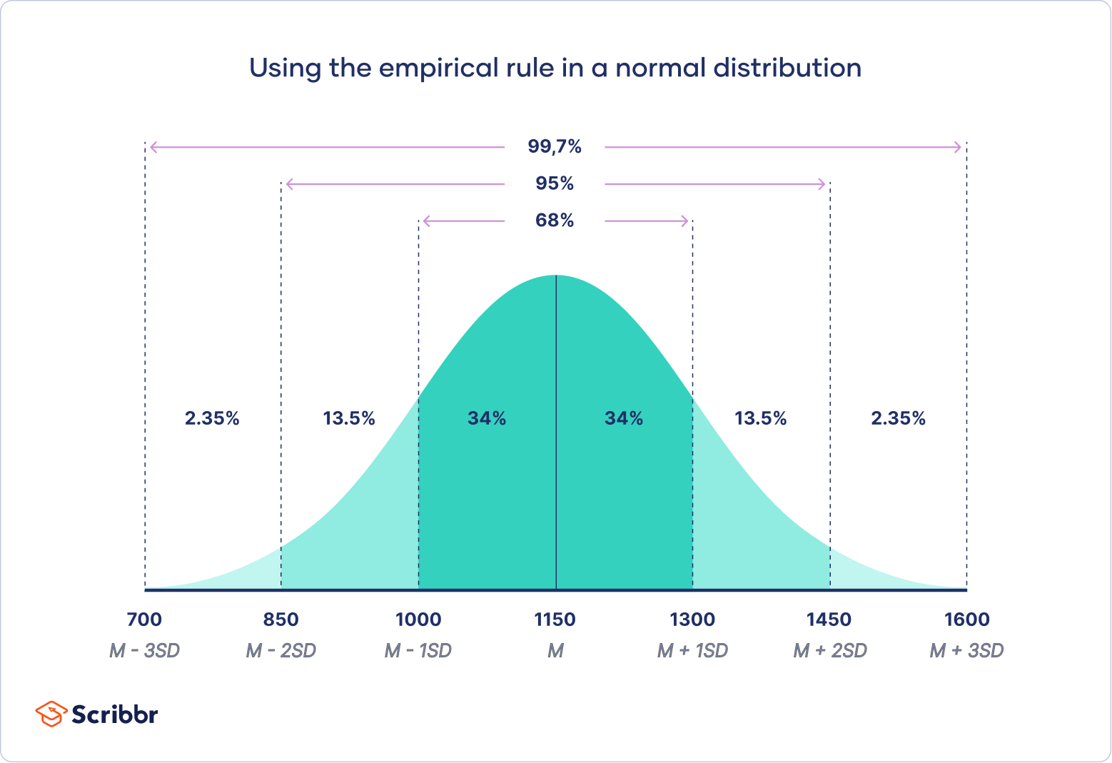
continuous, unimodal, symmetrical

N(u,o) mean and sd

Kertosis is

when the graph is too humpy or peaky , not spread out right

many real world variables are

normally distributed

z-score formula and the value formula:

z= (value-mean)/SD, use z-score to find prob/percentile

x= ZxSD+mean

to know whats to the right of a variable

do 1-the prob

to get the prob between two variables

get the prob of two and subtract the smaller one from the bigger