Prob/stats for biosciences EXAM 1 REVIEW

0.0(0)
Studied by 103 people
call kaiCall Kai
learnLearn
examPractice Test
spaced repetitionSpaced Repetition
heart puzzleMatch
flashcardsFlashcards
GameKnowt Play
Card Sorting

1/77

flashcard set

Earn XP

Description and Tags

I made this to help me study for the module exams! Hopefully it can help you guys too! I will fill this out through the duration of the course to prepare for each exam, by December this set should include every single topic of the course. ALSO, there are topics from the chapters included (some of which was not discussed in class!). I added some formulas separately from their topic, but all formulas are included in some flashcard, some are simply not separated on their own.

78 Terms

1
New cards

Descriptive Statistics

  • anything that describes/summarizes data (graphs, charts, etc.)


2
New cards

Inferential Statistics

  •  inferences about population based on sample (one that is representative of the entire population– testing)


3
New cards

Parameter

  • DESCRIBES POPULATION


4
New cards

Statistic

  • DESCRIBES SAMPLE


5
New cards

Simple Random Sampling (SRS)

  • ensures random selection → must be random or introduces BIAS 

    • -Every unit has SAME chance of being chosen 

    • -Sample size= n 

    • -Sample with replacement vs without replacement 


6
New cards

Variable

  • any characteristic, number, quantity, that can change from one to another 

    • Data being collected 

    • EX) age, income, eye color, gpa, etc.


7
New cards

DATA ANALYSIS PROCESS


  • Process of inspecting, transforming, cleansing, modeling data with the goal of finding useful PRACTICAL information (conclusions!)

1. Understanding nature of the problem

  • What are we trying to answer? Why perform this study?

2. Deciding measurement

  • What are we measuring, how do we measure it

3.Data Collection 

4.Data summarization and preliminary analysis 

  • DESCRIPTIVE STATS: graph, chart, table, numerical summary 

5. Formal Data Analysis

  • Hypothesis testing and estimation, confidence intervals→ inferential statistics 

6. Interpretation of results

  • Write about analysis, answering the research question from 1. 


8
New cards

Qualitative Data

Categorical Data: CATEGORIES

EX) eye color, major, class, etc.


9
New cards

Quantitative Data

Numerical Data

10
New cards

Quantitative Data: DISCRETE

  • whole number, count (number of blank)


11
New cards

Quantitative Data: CONTINUOUS

  • measurement (length, height, weight)


12
New cards

Graphing Techniques: FREQUENCY DISTRIBUTION

  • Frequency Distribution: summary table of the data

    • Frequencies: counts, how many of a certain value/response

      • Always a whole number

      • Displayed as “number of..”


13
New cards

Graphing Techniques: RELATIVE FREQUENCY

  • Relative frequencies: (frequency/total number of observations, sample size)

    • FORMULA (takes the frequency and divides by total # observations)

    • frequency/n

    • Also called PROPORTION!

    • DO NOT CONVERT INTO A PERCENT, only if asked to interpret results in terms of percentages

  • Before Graphing, must create a table to then graph


14
New cards

Graphing Techniques: BAR CHART

Visual representation of QUALITATIVE data

<p>Visual representation of QUALITATIVE data</p>
15
New cards

Graphing Techniques: COMPARATIVE BAR CHART

This is used in comparison of multiple variables (both MUST be qualitative variables in order to be a comparative bar chart) 


<p><span style="background-color: transparent; font-family: &quot;Century Gothic&quot;, sans-serif;">This is used in comparison of multiple variables (both MUST be qualitative variables in order to be a comparative bar chart)&nbsp;</span></p><p></p>
16
New cards

Graphing Techniques: PIE CHART

To visually represent QUALITATIVE data in form of relative frequencies or percentages
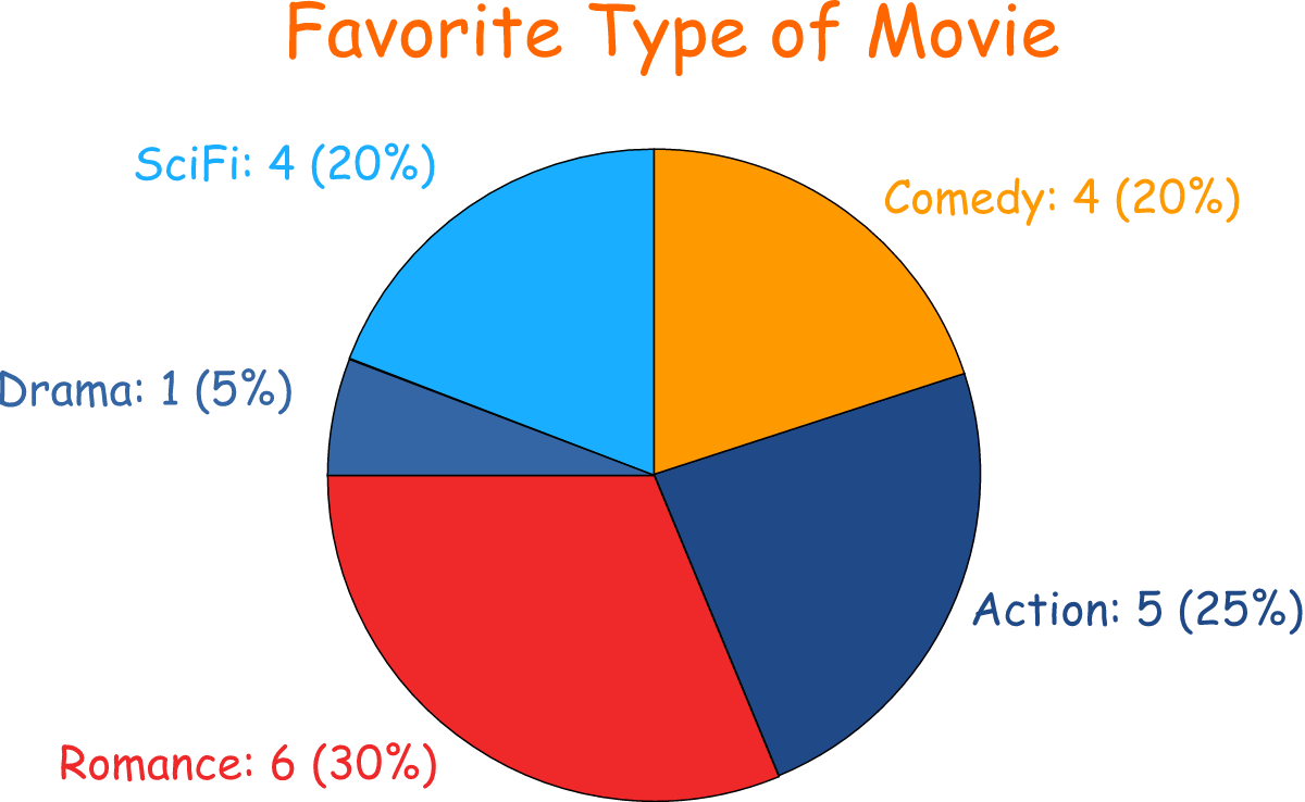
<p>To visually represent QUALITATIVE data in form of relative frequencies or percentages</p>
17
New cards

Graphing Techniques: HISTOGRAM

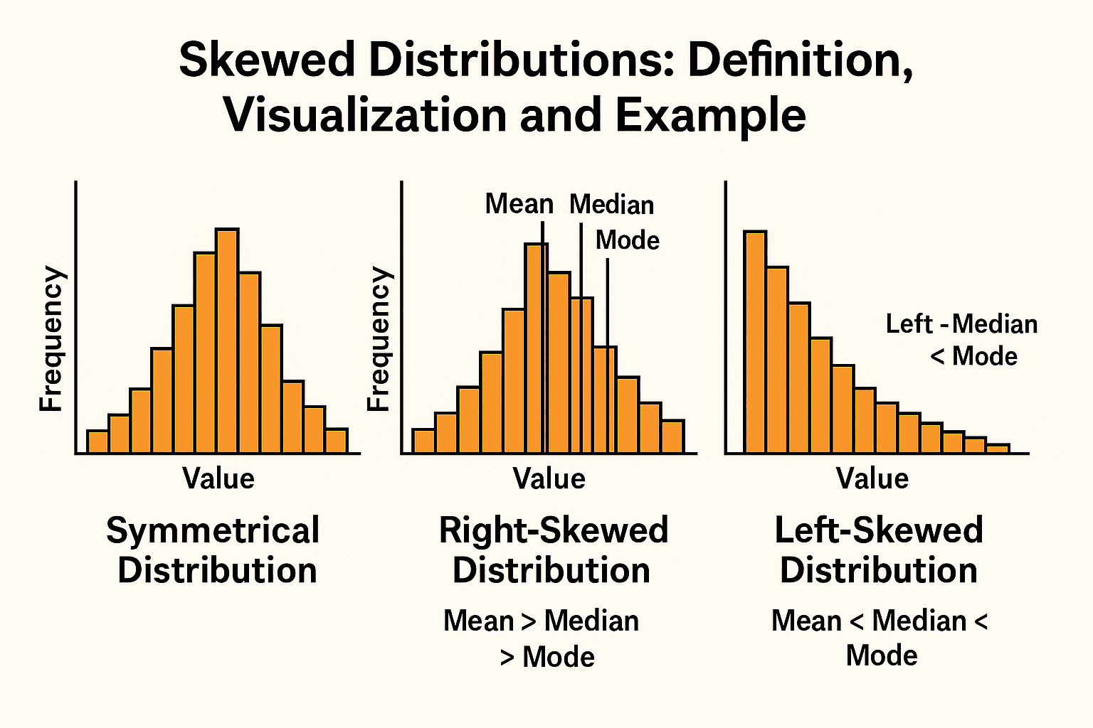
  • Bar chart for quantitative data, Data shown across MEANINGFUL intervals, ONLY One variable

  • SHAPES: 

    • -Symmetric (normal distribution, bell shaped curve)

      • mean and median will be exactly the same when data is symmetric SO typically use median for skewed due to outliers and range

    • -Skewed 

      • Skewed right (LONGER right tail, so peak is on the left) (POSITIVE skewed)

        • median stays in middle, the mean is larger

      • Skewed left (LONGER left tail, so peak is on the right) (NEGATIVE skewed)

        • median stays in middle, the mean is smaller

<ul><li><p><span style="background-color: transparent; font-family: &quot;Century Gothic&quot;, sans-serif;">Bar chart for quantitative data, Data shown across MEANINGFUL intervals, ONLY One variable</span></p></li></ul><ul><li><p><span style="background-color: transparent; font-family: &quot;Century Gothic&quot;, sans-serif;">SHAPES:&nbsp;</span></p><ul><li><p><span style="background-color: transparent; font-family: &quot;Century Gothic&quot;, sans-serif;">-Symmetric (normal distribution, bell shaped curve)</span></p><ul><li><p><span style="background-color: transparent;">mean and median will be exactly the same when data is symmetric SO typically use median for skewed due to outliers and range</span></p></li></ul></li><li><p><span style="background-color: transparent; font-family: &quot;Century Gothic&quot;, sans-serif;">-Skewed&nbsp;</span></p><ul><li><p><span style="background-color: transparent; font-family: &quot;Century Gothic&quot;, sans-serif;">Skewed right (LONGER right tail, so peak is on the left) (POSITIVE skewed)</span></p><ul><li><p><span style="background-color: transparent;">median stays in middle, the mean is larger</span></p></li></ul></li><li><p><span style="background-color: transparent; font-family: &quot;Century Gothic&quot;, sans-serif;">Skewed left (LONGER left tail, so peak is on the right) (NEGATIVE skewed)</span></p><ul><li><p><span style="background-color: transparent;">median stays in middle, the mean is smaller</span></p></li></ul></li></ul></li></ul></li></ul><p></p>
18
New cards

Graphing Techniques: SCATTERPLOT

  • points from two numerical values

    • Explanatory variable: the independent variable that predicts the outcome, x-axis

    • Response variable: the dependent variable (outcome of interest), y-axis

    • This will be linked with a RESEARCH QUESTION, which will tell you which variable is explanatory/response


<ul><li><p><span style="background-color: transparent; font-family: &quot;Century Gothic&quot;, sans-serif;">points from two numerical values</span></p><ul><li><p><span style="background-color: transparent; font-family: &quot;Century Gothic&quot;, sans-serif;"><strong>Explanatory </strong>variable: the independent variable that predicts the outcome, x-axis</span></p></li><li><p><span style="background-color: transparent; font-family: &quot;Century Gothic&quot;, sans-serif;"><strong>Response </strong>variable: the dependent variable (outcome of interest), y-axis</span></p></li><li><p><span style="background-color: transparent; font-family: &quot;Century Gothic&quot;, sans-serif;">This will be linked with a RESEARCH QUESTION, which will tell you which variable is explanatory/response</span></p></li></ul></li></ul><p></p>
19
New cards

Graphing Techniques: DOT PLOT

  • Each data value is plotted as a point above a horizontal scale of values, dots representing equal stacked values 

    • Displays shape of distribution of data

    • JITTER: randomly nudges points so that they don't overlap, instead of identical data values being plotted on top, allows to see separate points that are close together


<ul><li><p><span style="background-color: transparent; font-family: &quot;Century Gothic&quot;, sans-serif;">Each data value is plotted as a point above a horizontal scale of values, dots representing equal stacked values&nbsp;</span></p><ul><li><p><span style="background-color: transparent; font-family: &quot;Century Gothic&quot;, sans-serif;">Displays shape of distribution of data</span></p></li><li><p><span style="background-color: transparent; font-family: &quot;Century Gothic&quot;, sans-serif;">JITTER: randomly nudges points so that they don't overlap, instead of identical data values being plotted on top, allows to see separate points that are close together</span></p></li></ul></li></ul><p></p>
20
New cards

Graphing Techniques: STEM PLOT

  •  Separating each value into two parts: STEM (leftmost digit) and the LEAF (rightmost digit)

    • Shows shape of the distribution data 

    • Retains original data values 

    • Sample data are sorted/arranged in order 


<ul><li><p><span style="background-color: transparent; font-family: &quot;Century Gothic&quot;, sans-serif;"><strong>&nbsp;</strong>Separating each value into two parts: STEM (leftmost digit) and the LEAF (rightmost digit)</span></p><ul><li><p><span style="background-color: transparent; font-family: &quot;Century Gothic&quot;, sans-serif;">Shows shape of the distribution data&nbsp;</span></p></li><li><p><span style="background-color: transparent; font-family: &quot;Century Gothic&quot;, sans-serif;">Retains original data values&nbsp;</span></p></li><li><p><span style="background-color: transparent; font-family: &quot;Century Gothic&quot;, sans-serif;">Sample data are sorted/arranged in order&nbsp;</span></p></li></ul></li></ul><p></p>
21
New cards

Measures of Center: SAMPLE MEAN

  • (AKA average): sum of all observations in a dataset divided by total number observations (sample size) 

    • Lowercase letters as observations for the variable (lowercase x=variable, so you don't have to write the variable out)


<ul><li><p><span style="background-color: transparent; font-family: &quot;Century Gothic&quot;, sans-serif;">(AKA average): sum of all observations in a dataset divided by total number observations (sample size)&nbsp;</span></p><ul><li><p><span style="background-color: transparent; font-family: &quot;Century Gothic&quot;, sans-serif;">Lowercase letters as observations for the variable (lowercase x=variable, so you don't have to write the variable out)</span></p></li></ul></li></ul><p></p>
22
New cards

Measures of Center: SAMPLE MEDIAN

  • middle value in an ordered dataset

    • -Dataset MUST be ordered, smallest to largest!!!

    • -When n is ODD, we have a unique median: one SINGLE value in the very middle of our dataset

    • -When n is EVEN, we will average the 2 middle values!! (Basically between the 2 values)


23
New cards

Measures of Center: SAMPLE MODE

  • the value(s) that occur most frequently in a dataset 

    • UNIMODAL: one mode, BIMODAL: 2 modes, MULTIMODAL: multiple modes


24
New cards

Measures of Spread: RANGE

  •  maximum-minimum (single value that summarizes our data)


25
New cards

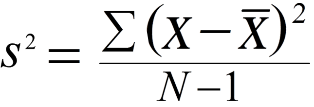
Measures of Spread: SAMPLE VARIANCE

  • a measure of how spread out the data is relative to the mean 

    • Deviation from the mean→ How FAR a single value is from the mean, xᵢ - x̄ 

    • When xi is smaller than mean= negative value, when xi larger than mean=positive value

    • The NUMERATOR; sum all deviations from the means WILL ALWAYS EQUAL 0.. Which is why we use variance with the squared numerator→ it gets rid of those negative differences so that we don’t end up with 0


    • -UNIT IS SQUARED 

    • -Sample variance = (standard deviation) ^2

<ul><li><p><span style="background-color: transparent; font-family: &quot;Century Gothic&quot;, sans-serif;">a measure of how spread out the data is relative to the mean&nbsp;</span></p><ul><li><p><span style="background-color: transparent; font-family: &quot;Century Gothic&quot;, sans-serif;">Deviation from the mean→ How FAR a single value is from the mean, <strong>xᵢ - </strong>x̄<strong>&nbsp;</strong></span></p></li><li><p><span style="background-color: transparent; font-family: &quot;Century Gothic&quot;, sans-serif;">When xi is smaller than mean= negative value, when xi larger than mean=positive value</span></p></li><li><p><span style="background-color: transparent; font-family: &quot;Century Gothic&quot;, sans-serif;">The NUMERATOR; sum all deviations from the means WILL ALWAYS EQUAL 0.. Which is why we use variance with the squared numerator→ it gets rid of those negative differences so that we don’t end up with 0</span></p></li><li><p></p></li><li><p><span style="background-color: transparent; font-family: &quot;Century Gothic&quot;, sans-serif;">-UNIT IS SQUARED&nbsp;</span></p></li><li><p><span style="background-color: transparent; font-family: &quot;Century Gothic&quot;, sans-serif;">-Sample variance = (standard deviation) ^2</span></p></li></ul></li></ul><p></p>
26
New cards

Measures of Spread: SAMPLE STANDARD DEVIATION (SD)

  • Getting rid of those squared units→ to get sample deviation 

—> CAN JUST SQUARE ROOT THE SAMPLE VARIANCE

<ul><li><p><span style="background-color: transparent; font-family: &quot;Century Gothic&quot;, sans-serif;">Getting rid of those squared units→ to get sample deviation&nbsp;</span></p></li></ul><p><span style="background-color: transparent; font-family: &quot;Century Gothic&quot;, sans-serif;">—&gt; CAN JUST SQUARE ROOT THE SAMPLE VARIANCE</span></p>
27
New cards

IMPORTANT TIP!

  • When performing calculations by hand, use as many decimals as possible (minimum of 5-6 decimals to get exact values), the more the better!


28
New cards

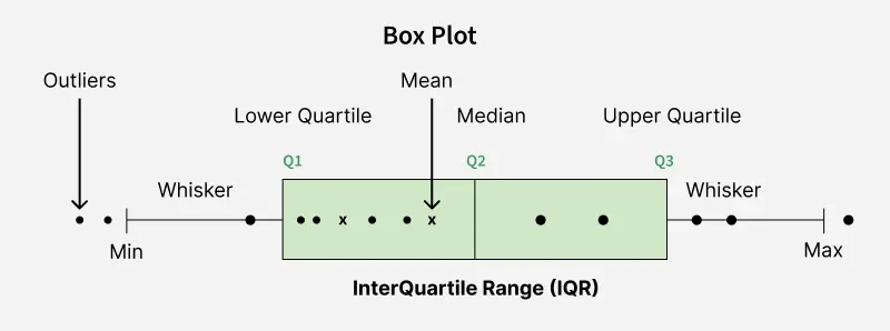
Box and Whisker plot/boxplot

  • graphical display that summarizes information about center, spread, symmetry, skewness of data

    • INTERPRETATIONS: center of distribution, shape of distribution, variability of distribution, useful for making comparisons across several groups of data

  • MAKE SURE DATA IS ORDERED!! IF IT IS NOT, ORDER IT!


<ul><li><p><span style="background-color: transparent; font-family: &quot;Century Gothic&quot;, sans-serif;">graphical display that summarizes information about center, spread, symmetry, skewness of data</span></p><ul><li><p><span style="background-color: transparent; font-family: &quot;Century Gothic&quot;, sans-serif;">INTERPRETATIONS: center of distribution, shape of distribution, variability of distribution, useful for making comparisons across several groups of data</span></p></li></ul></li><li><p><span style="background-color: transparent; font-family: &quot;Century Gothic&quot;, sans-serif;">MAKE SURE DATA IS ORDERED!! IF IT IS NOT, ORDER IT!</span></p></li></ul><p></p>
29
New cards

Five Number Summary

Used in interpreting and creating Box and Whisker plot/boxplot.

1.Minimum

2.1st Quartile (Q1)- 25th percentile of an ordered dataset

3. 2nd Quartile (Q2)- 50th percentile of an ordered dataset

4.3rd Quartile (Q3)- 75th percentile of an ordered dataset

5.Maximum


30
New cards

Percentiles

Commonly seen in Five Number Summary/Whisker plots

  • Percentiles: the value at which p% of the data fall AT or BELOW 

    • -p= what percentile you are interested in

    • -Integer= whole number

    • -FORMULA: np/100


    • ******If np/100 is not an integer, the observation is greater than the (np/100)th placement (use the next whole value)

    • ******If np/100 is an integer, the average of the (np/100)th and (np/100 + 1)th observations


EX)  3, 8, 10, 14, 20, 30            n=6, find the 50th percentile, P50

  • np/100= 6(50)/100= 3 ← AN INTEGER —> AVERAGE OF THAT VALUE AND THE NEXT VALUE, average the 3rd and 4th values

   -  (10+14)/2 = 12 = 50th percentile


31
New cards

Interquartile range (IQR)

Used exclusively in Whisker plots and five number summaries

  • we have an interquartile range: IQR= Q3-Q1

    • Q1= 25th percentile 

    • Q3 = 75th percentile 

    • This gives the range of the middle half of the data→ another measure of spread we discuss when we interpret the box and whisker plot 

    • IQR helps us calculate outliers …

  • UPPER whisker: Q3 + 1.5(IQR) → if calculated value is smaller, than use the calculated value as max and any value above is an outlier

  • LOWER whisker: Q1 - 1.5(IQR) → if the calculated value is larger, the calculated value is the new minimum

<p>Used exclusively in Whisker plots and five number summaries</p><ul><li><p><span style="background-color: transparent; font-family: &quot;Century Gothic&quot;, sans-serif;">we have an interquartile range:<strong><mark data-color="#fafa8a" style="background-color: rgb(250, 250, 138); color: inherit;"> IQR= Q3-Q1</mark></strong></span></p><ul><li><p><span style="background-color: transparent; font-family: &quot;Century Gothic&quot;, sans-serif;">Q1= 25th percentile&nbsp;</span></p></li><li><p><span style="background-color: transparent; font-family: &quot;Century Gothic&quot;, sans-serif;">Q3 = 75th percentile&nbsp;</span></p></li><li><p><span style="background-color: transparent; font-family: &quot;Century Gothic&quot;, sans-serif;">This gives the range of the middle half of the data→ another measure of spread we discuss when we interpret the box and whisker plot&nbsp;</span></p></li><li><p><span style="background-color: transparent; font-family: &quot;Century Gothic&quot;, sans-serif;">IQR helps us calculate outliers …</span></p></li></ul></li><li><p><span style="background-color: transparent; font-family: &quot;Century Gothic&quot;, sans-serif;"><strong>UPPER whisker: <mark data-color="#ffe670" style="background-color: rgb(255, 230, 112); color: inherit;">Q3 + 1.5(IQR)</mark> → if calculated value is smaller, than use the calculated value as max and any value above is an outlier</strong></span></p></li><li><p><span style="background-color: transparent; font-family: &quot;Century Gothic&quot;, sans-serif;"><strong>LOWER whisker: <mark data-color="#fae87b" style="background-color: rgb(250, 232, 123); color: inherit;">Q1 - 1.5(IQR) </mark>→ if the calculated value is larger, the calculated value is the new minimum</strong></span></p></li></ul><p></p>
32
New cards

Outliers in data

  • Outliers: observation that differs significantly from other observations in a random sample of data

33
New cards
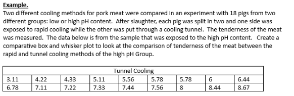
<p>Example Problem: Solve for the Five Number Summary, calculate any outliers, and draw the whisker plot!</p>

Example Problem: Solve for the Five Number Summary, calculate any outliers, and draw the whisker plot!

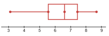
 5 number summary 

  1. Minimum: 3.11 

  2. Q1: NP/100 → (18(25))/100= 4.5 → NOT AN INTEGER, next value up is the fifth one

    1. Q1=  5.56

  3. Q2: NP/100 → (18(50))/100= 9 → INTEGER, average the ninth and tenth values in data set

    1. Q2: (6.44 +6.78)/2 = 6.61

  4. Q3: NP/100 → (18(75))/100= 13.5 → NOT INTEGER< use fourteenth value

    1. Q3: 7.44 

  5. Maximum: 8.67


Now we need to determine if there are outliers/extreme values in our dataset!!!! 

  • UPPER whisker: Q3 + 1.5(IQR) → set at MAX if larger 

  • LOWER whisker: Q1 - 1.5(IQR) → set at MIN if smaller

  • IQR= Q3-Q1

  • Lower whisker: Q1- 1.5(IQR) 

(5.56)-1.5(7.44-5.56)= 2.74 

THIS VALUE IS LOWER THAN THE MINIMUM→The minimum is higher than the whisker, therefore we simply draw the lower whisker at the minimum

  • THIS TELLS US WE HAVE NO OUTLIERS ON LOWER END!

  • Upper whisker: Q3+1.5(IQR)

(7.44)+1.5(7.44-5.56)= 10.26

THIS VALUE IS THAN HIGHER THE MAXIMUM→ The maximum is lower than the whisker value, therefore we simply draw the upper whisker at the maximum 

  • THIS TELLS US WE HAVE NO OUTLIERS ON THE UPPER END! 


Whisker plot seen: LABEL AXES!

X axis: tenderness of meat

Y axis: Tunnel Cooling method


<p><span style="background-color: transparent; font-family: &quot;Century Gothic&quot;, sans-serif;">&nbsp;5 number summary&nbsp;</span></p><ol><li><p><span style="background-color: transparent; font-family: &quot;Century Gothic&quot;, sans-serif;">Minimum: <strong>3.11&nbsp;</strong></span></p></li><li><p><span style="background-color: transparent; font-family: &quot;Century Gothic&quot;, sans-serif;">Q1: NP/100 → (18(25))/100= 4.5 → NOT AN INTEGER, next value up is the fifth one</span></p><ol><li><p><span style="background-color: transparent; font-family: &quot;Century Gothic&quot;, sans-serif;">Q1=&nbsp; <strong>5.56</strong></span></p></li></ol></li><li><p><span style="background-color: transparent; font-family: &quot;Century Gothic&quot;, sans-serif;">Q2: NP/100 → (18(50))/100= 9 → INTEGER, average the ninth and tenth values in data set</span></p><ol><li><p><span style="background-color: transparent; font-family: &quot;Century Gothic&quot;, sans-serif;">Q2: (6.44 +6.78)/2 = <strong>6.61</strong></span></p></li></ol></li><li><p><span style="background-color: transparent; font-family: &quot;Century Gothic&quot;, sans-serif;">Q3: NP/100 → (18(75))/100= 13.5 → NOT INTEGER&lt; use fourteenth value</span></p><ol><li><p><span style="background-color: transparent; font-family: &quot;Century Gothic&quot;, sans-serif;">Q3: <strong>7.44&nbsp;</strong></span></p></li></ol></li><li><p><span style="background-color: transparent; font-family: &quot;Century Gothic&quot;, sans-serif;">Maximum: <strong>8.67</strong></span></p></li></ol><p><br></p><p><span style="background-color: transparent; font-family: &quot;Century Gothic&quot;, sans-serif;">Now we need to determine if there are outliers/extreme values in our dataset!!!!&nbsp;</span></p><ul><li><p><span style="background-color: transparent; font-family: &quot;Century Gothic&quot;, sans-serif;">UPPER whisker: Q3 + 1.5(IQR) → set at MAX if larger&nbsp;</span></p></li><li><p><span style="background-color: transparent; font-family: &quot;Century Gothic&quot;, sans-serif;">LOWER whisker: Q1 - 1.5(IQR) → set at MIN if smaller</span></p></li><li><p><span style="background-color: transparent; font-family: &quot;Century Gothic&quot;, sans-serif;">IQR= Q3-Q1</span></p></li></ul><ul><li><p><span style="background-color: transparent; font-family: &quot;Century Gothic&quot;, sans-serif;">Lower whisker: Q1- 1.5(IQR)&nbsp;</span></p></li></ul><p><span style="background-color: transparent; font-family: &quot;Century Gothic&quot;, sans-serif;">(5.56)-1.5(7.44-5.56)= <strong>2.74&nbsp;</strong></span></p><p><span style="background-color: transparent; font-family: &quot;Century Gothic&quot;, sans-serif;">THIS VALUE IS LOWER THAN THE MINIMUM→The minimum is higher than the whisker, therefore we simply draw the lower whisker at the minimum</span></p><ul><li><p><span style="background-color: transparent; font-family: &quot;Century Gothic&quot;, sans-serif;">THIS TELLS US WE HAVE NO OUTLIERS ON LOWER END!</span></p></li></ul><ul><li><p><span style="background-color: transparent; font-family: &quot;Century Gothic&quot;, sans-serif;">Upper whisker: Q3+1.5(IQR)</span></p></li></ul><p><span style="background-color: transparent; font-family: &quot;Century Gothic&quot;, sans-serif;">(7.44)+1.5(7.44-5.56)=<strong> 10.26</strong></span></p><p><span style="background-color: transparent; font-family: &quot;Century Gothic&quot;, sans-serif;">THIS VALUE IS THAN HIGHER THE MAXIMUM→ The maximum is lower than the whisker value, therefore we simply draw the upper whisker at the maximum&nbsp;</span></p><ul><li><p><span style="background-color: transparent; font-family: &quot;Century Gothic&quot;, sans-serif;">THIS TELLS US WE HAVE NO OUTLIERS ON THE UPPER END!&nbsp;</span></p></li></ul><p></p><p>Whisker plot seen: LABEL AXES! </p><p><span style="background-color: transparent; font-family: &quot;Century Gothic&quot;, sans-serif;">X axis: tenderness of meat</span></p><p><span style="background-color: transparent; font-family: &quot;Century Gothic&quot;, sans-serif;">Y axis: Tunnel Cooling method</span></p><p></p><p></p>
34
New cards

Probability

  • The likelihood of an occurrence of some outcome, from a chance experiment : “How likely something is to happen” 

  • We have to have data probabilities to support and defend our answer


  • All probabilities must be between 0 and 1

    • 0≤ P(A)≤ 1

  • All probabilities in the sample space MUST sum to 1 


35
New cards

Event

  • outcome(s) from a chance experiment 

    • examples: tossing a coin, card games, etc.

    • Toss a coin: let A = the event that we toss a tail


  • Compound event: any event combining 2+ simple events

**We typically use capitals as variables to define events


36
New cards

Sample Space

  •  List of all possible outcomes from a chance experiment

    • ex) tossing a coin two times; 

      • List of all possible outcomes: HH, HT, TH, TT

      • Allows us to determine the total number of outcomes from a chance experiment, which equates to helping us compute probabilities 


37
New cards

Classical Method of Probability

  • Let A be an event from a chance experiment, then: 

    • P(A)= (# times A occurs / total # of outcomes) → The probability of event A


    • ex) toss a coin 2 times, what is the probability it lands on tails both times? 

      • Let A= tossing tail on 2 tosses

      • List of all possible outcomes: HH, HT, TH, TT

      • Denominator= 4, there's 4 possible outcomes, how many times event A occurs is ONCE → ¼ =probability of landing tails twice when tossing that coin twice


<ul><li><p><span style="background-color: transparent; font-family: &quot;Century Gothic&quot;, sans-serif;">Let A be an event from a chance experiment, then:&nbsp;</span></p><ul><li><p><span style="background-color: transparent; font-family: &quot;Century Gothic&quot;, sans-serif;">P(A)= (# times A occurs / total # of outcomes) → The probability of event A</span></p></li><li><p></p></li><li><p><span style="background-color: transparent; font-family: &quot;Century Gothic&quot;, sans-serif;">ex) toss a coin 2 times, what is the probability it lands on tails both times?&nbsp;</span></p><ul><li><p><span style="background-color: transparent; font-family: &quot;Century Gothic&quot;, sans-serif;">Let A= tossing tail on 2 tosses</span></p></li><li><p><span style="background-color: transparent; font-family: &quot;Century Gothic&quot;, sans-serif;">List of all possible outcomes: HH, HT, TH, TT</span></p></li><li><p><span style="background-color: transparent; font-family: &quot;Century Gothic&quot;, sans-serif;">Denominator= 4, there's 4 possible outcomes, how many times event A occurs is ONCE → ¼ =probability of landing tails twice when tossing that coin twice</span></p></li></ul></li></ul></li></ul><p></p>
38
New cards

Complex events: INTERSECTION of events

  • When both events A and B occur at the same time 

  • P(A∩B)

  • = (# times A AND B occur) / (total # outcomes)

  • The middle of circles in Venn diagram 


AKA JOINT PROBABILITY

—OUT OF THE TOTAL ON CONTINGENCY TABLES


***ON CONTINGENCY TABLES THIS WILL BE THE VALUES OF ROWS AND COLUMNS INTERSECTING!


<ul><li><p><span style="background-color: transparent; font-family: &quot;Century Gothic&quot;, sans-serif;">When both events A and B occur at the same time&nbsp;</span></p></li><li><p><span style="background-color: transparent; font-family: &quot;Century Gothic&quot;, sans-serif;">P(A∩B)</span></p></li><li><p><span style="background-color: transparent; font-family: &quot;Century Gothic&quot;, sans-serif;">= (# times A AND B occur) / (total # outcomes)</span></p></li><li><p><span style="background-color: transparent; font-family: &quot;Century Gothic&quot;, sans-serif;">The middle of circles in Venn diagram&nbsp;</span></p></li></ul><p></p><p>AKA <strong>JOINT </strong>PROBABILITY </p><p>—OUT OF THE TOTAL ON CONTINGENCY TABLES</p><p></p><p>***ON CONTINGENCY TABLES THIS WILL BE THE VALUES OF ROWS AND COLUMNS INTERSECTING!</p><p><br></p>
39
New cards

Complex events: UNION of events

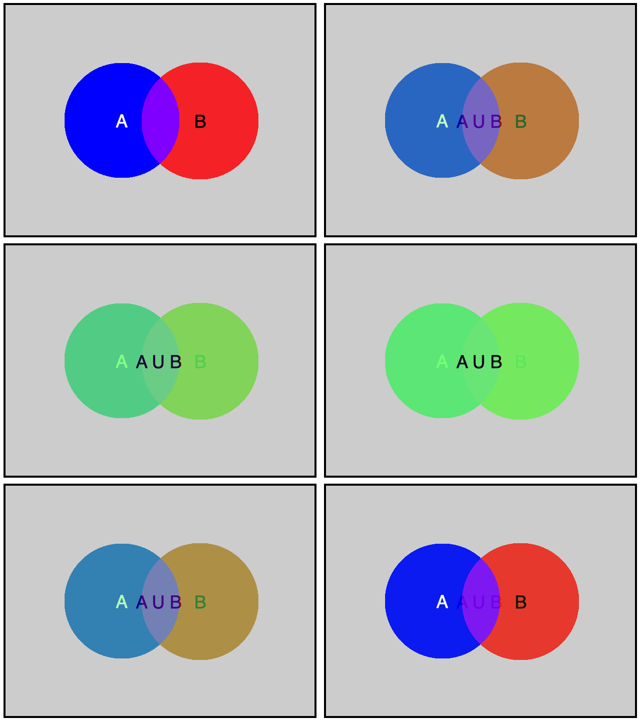
  • When either event A or event B or both events occur 

  • P(A∪B)

  • Interested in the ENTIRETY of the circles; A or B or BOTH ! 

  • THE ADDITIVE RULE:

    • P(A) + P(B) - P(A∩B)

    • The reason we need to subtract intersection is so we don't double dip! 

<ul><li><p><span style="background-color: transparent; font-family: &quot;Century Gothic&quot;, sans-serif;">When either event A or event B <strong>or </strong>both events occur&nbsp;</span></p></li><li><p><span style="background-color: transparent; font-family: &quot;Century Gothic&quot;, sans-serif;">P(A∪B)</span></p></li></ul><ul><li><p><span style="background-color: transparent; font-family: &quot;Century Gothic&quot;, sans-serif;">Interested in the ENTIRETY of the circles; A or B or BOTH !&nbsp;</span></p></li><li><p><span style="background-color: transparent; font-family: &quot;Century Gothic&quot;, sans-serif;"><strong>THE ADDITIVE RULE:</strong></span></p><ul><li><p><span style="background-color: transparent; font-family: &quot;Century Gothic&quot;, sans-serif;">P(A) + P(B) - P(A∩B)</span></p></li><li><p><span style="background-color: transparent; font-family: &quot;Century Gothic&quot;, sans-serif;">The reason we need to subtract intersection is so we don't double dip!&nbsp;</span></p></li></ul></li></ul><p></p>
40
New cards

Complex events: COMPLEMENT of events

  • Complement of event A is everything in the sample space except event A

  • - Denoted as: P(A^c) OR P(A bar)


  • To find the probability of the complement: 

    • P(A c)= 1 - P(A) **and vice versa

    • P(A) + P(Ac)=1


<ul><li><p><span style="background-color: transparent; font-family: &quot;Century Gothic&quot;, sans-serif;">Complement of event A is everything in the sample space except event A</span></p></li><li><p><span style="background-color: transparent; font-family: &quot;Century Gothic&quot;, sans-serif;">- Denoted as: P(A^c) OR P(A bar)</span></p></li><li><p></p></li></ul><ul><li><p><span style="background-color: transparent; font-family: &quot;Century Gothic&quot;, sans-serif;">To find the probability of the complement:&nbsp;</span></p><ul><li><p><span style="background-color: transparent; font-family: &quot;Century Gothic&quot;, sans-serif;">P(A c)= 1 - P(A) **and vice versa</span></p></li><li><p><span style="background-color: transparent; font-family: &quot;Century Gothic&quot;, sans-serif;">P(A) + P(Ac)=1</span></p></li></ul></li></ul><p></p>
41
New cards

Mutually Exclusive Events

  • 2 events CANNOT HAPPEN simultaneously 

    • Ex) tossing a coin; cannot land on heads or tails at the same time= mutually exclusive events 

    • These are DISJOINT events 


  • P(A∪B)= P(A) + P(B)    ← no intersection between events 

  • P(A∩B)= 0


<ul><li><p><span style="background-color: transparent; font-family: &quot;Century Gothic&quot;, sans-serif;">2 events CANNOT HAPPEN simultaneously&nbsp;</span></p><ul><li><p><span style="background-color: transparent; font-family: &quot;Century Gothic&quot;, sans-serif;">Ex) tossing a coin; cannot land on heads or tails at the same time= mutually exclusive events&nbsp;</span></p></li><li><p><span style="background-color: transparent; font-family: &quot;Century Gothic&quot;, sans-serif;">These are DISJOINT events&nbsp;</span></p></li><li><p></p></li></ul></li></ul><ul><li><p><span style="background-color: transparent; font-family: &quot;Century Gothic&quot;, sans-serif;">P(A∪B)= P(A) + P(B)&nbsp; &nbsp; ← no intersection between events&nbsp;</span></p></li><li><p><span style="background-color: transparent; font-family: &quot;Century Gothic&quot;, sans-serif;">P(A∩B)= 0</span></p></li></ul><p></p>
42
New cards

Independent Events

  • probability of one event does NOT affect the probability of another event 

    • Ex) Coin toss; tossing the coin first getting heads, does not influence what we get on the next coin toss 

  • When events are independent: 

    • P(A∩B)= P(A) x P(B) → P(A) x P(B|A)


<ul><li><p><span style="background-color: transparent; font-family: &quot;Century Gothic&quot;, sans-serif;">probability of one event does NOT affect the probability of another event&nbsp;</span></p><ul><li><p><span style="background-color: transparent; font-family: &quot;Century Gothic&quot;, sans-serif;">Ex) Coin toss; tossing the coin first getting heads, does not influence what we get on the next coin toss&nbsp;</span><br></p></li></ul></li></ul><ul><li><p><span style="background-color: transparent; font-family: &quot;Century Gothic&quot;, sans-serif;">When events are independent:&nbsp;</span></p><ul><li><p><span style="background-color: transparent; font-family: &quot;Century Gothic&quot;, sans-serif;">P(A∩B)= P(A) x P(B) → P(A) x P(B|A)</span></p></li></ul></li></ul><p></p>
43
New cards

Conditional Probability

  • Probability of one event given another event has already occurred 

  • Changes what you are dividing by, the event that was given is what you are dividing by!!


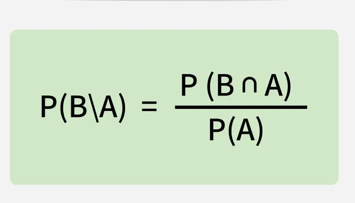
  • P(A|B)= P(A n B) / P(B)

    • The probability of event A given event BP(B|A):

    • the probability of event B occurring after event A already occurred


<ul><li><p><span style="background-color: transparent; font-family: &quot;Century Gothic&quot;, sans-serif;">Probability of one event given another event has already occurred&nbsp;</span></p></li><li><p><span style="background-color: transparent; font-family: &quot;Century Gothic&quot;, sans-serif;">Changes what you are dividing by, the event that was given is what you are dividing by!!</span></p></li><li><p></p></li><li><p><span style="background-color: transparent; font-family: &quot;Century Gothic&quot;, sans-serif;">P(A|B)= P(A n B) / P(B)</span></p><ul><li><p><span style="background-color: transparent; font-family: &quot;Century Gothic&quot;, sans-serif;">The probability of event A given event BP(B|A): </span></p></li><li><p><span style="background-color: transparent; font-family: &quot;Century Gothic&quot;, sans-serif;">the probability of event B occurring after event A already occurred</span></p></li></ul></li><li><p></p></li></ul><p></p>
44
New cards

Marginal Probability

  • The probability of a single event in a chance experiment 

  • P(A)= # times A occurs / total # outcomes


AKA CLASSICAL PROBABILITY METHOD


45
New cards

Contingency table

  • A 2 way table summarizing events of interest in a chance experiment

  • R X C (Row events, Column events)


***REC MAKING ONE IN PROBABILITY PROBLEMS!


<ul><li><p><span style="background-color: transparent; font-family: &quot;Century Gothic&quot;, sans-serif;">A 2 way table summarizing events of interest in a chance experiment</span></p></li><li><p><span style="background-color: transparent; font-family: &quot;Century Gothic&quot;, sans-serif;">R X C (Row events, Column events)</span></p></li></ul><p></p><p>***REC MAKING ONE IN PROBABILITY PROBLEMS!</p><p></p>
46
New cards
<p>Practice!</p><p>1.What is the total amount of people surveyed?</p><p>2. What kind of data is presented? (Qualitative,Quantitative,Categorical,Numerical,etc.)?</p><p>3.What is the probability of randomly selecting a person that has blue eyes?</p><p>4.What is the probability of randomly selecting a male with green eyes?</p><p>5.What is the probability of selecting a female or a someone with black eyes or both?</p><p>6.What is the probability of selecting a male given that they have gray eyes?</p><p></p>

Practice!

1.What is the total amount of people surveyed?

2. What kind of data is presented? (Qualitative,Quantitative,Categorical,Numerical,etc.)?

3.What is the probability of randomly selecting a person that has blue eyes?

4.What is the probability of randomly selecting a male with green eyes?

5.What is the probability of selecting a female or a someone with black eyes or both?

6.What is the probability of selecting a male given that they have gray eyes?


1.167 people were surveyed. —>Look at the summation of the totals!
2.Qualitative Categorical Data —> Eye color is the variable, which is a category!

3.This is a marginal probability P(A), We will call this P(B) for blue eyes. P(B)= number of people with blue eyes/total number of people —> 22/167 = 0.1317..

4.This is Intersection of events: P(A and B), we will call this P(M and G) = number of times males have green eyes / total number of people—> 20/167 = 0.11976…

5. This is a Unity of events; event A or event B or both; P(A) + P(B) - P(A n B) —> P(F) + P(B) - P(F n B)= (85/167) + (45/167) - (20/167) = 0.6586..

6. This is Conditional Probability: P(A|B)= P(A n B) / P(A) —>

P(M|G)= P(Male and Gray eyes) / P(Gray) = (10/167) / (20/167)= 0.50


47
New cards

PROBABILITY TIP!

Think of P(A n B) as A AND B, N = INtersection

48
New cards

Screening Tests: SENSITIVITY

  • Sensitivity: Probability that a diagnostic test will show a correct result (positive) if the individual has the disease 

    • If the individual has the disease→ this is the given event 

    • P(Positive|Disease)

    • We want this value to be high!


49
New cards

Screening tests: SPECIFICITY

  •  Probability that a diagnostic test will show a correct result (negative) if no disease is present 

    • If the individual does not have the disease→ this is the given event 

    • P(Negative|No disease) 

    • We want this value to be high!


50
New cards

Screening tests: PREDICTIVE VALUE POSITIVE (PV+)

  • The probability that a person has the disease GIVEN that the test is positive 

    • P(Disease|Positive) 

    • Inverse of Sensitivity, different probabilities because given event is different 

    • ONLY out of the positive results, how many have the disease 


51
New cards

Screening tests: PREDICTIVE VALUE NEGATIVE (PV-)

  • Probability that a person does not have a disease GIVEN that the test is negative 

    • P(No disease|Negative) 

    • Inverse of Specificity, different probabilities because given event is different 

    • ONLY out of the negative results, how many do not have the disease 


52
New cards

Screening tests: FALSE POSITIVE

  • probability of a positive test result when the disease is not present 

    • P(Positive|No disease)


53
New cards

Screening tests: FALSE NEGATIVE

  •  probability of a negative test result when the disease is present 

    • P(Negative|Disease)


54
New cards

Baye’s Theorem

  • Allows us to use P(A|B) to calculate P(B|A)

    • NOTE: P(A|B) = P(A n B)/P(B) → Bayes theory rearranges this formula to solve for joint probability 

      • P(A n B) = P(A|B) x P(B) —> use when solving with contingency table!


<ul><li><p><span style="background-color: transparent; font-family: &quot;Century Gothic&quot;, sans-serif;">Allows us to use P(A|B) to calculate P(B|A)</span></p><ul><li><p><span style="background-color: transparent; font-family: &quot;Century Gothic&quot;, sans-serif;">NOTE: P(A|B) = P(A n B)/P(B) → Bayes theory rearranges this formula to solve for joint probability&nbsp;</span></p><ul><li><p><span style="background-color: transparent; font-family: &quot;Century Gothic&quot;, sans-serif;"><strong><mark data-color="#fff184" style="background-color: rgb(255, 241, 132); color: inherit;">P(A n B) = P(A|B) x P(B) —&gt; </mark></strong>use when solving with contingency table!</span></p></li></ul></li></ul></li></ul><p></p>
55
New cards
<p>Example of Baye’s Theorem: </p>

Example of Baye’s Theorem:

  • Start with givens 

    • D= Tuberculosis ND=Not have Tuberculosis 

  • Sensitivity: positive and has disease→ P(positive|D)= .95

    • CONDITIONALS MUST BE USED TO FIND INTERSECTION!!!!!! .95 CANNOT BE PUT INTO THE TABLE, NEED TO SOLVE FOR JOINT PROBABILITY WITH BAYES THEOREM 

      • P(Positive n Disease) = P(positive|Disease) x P(Disease) = 0.95 x 0.20 =0.19

  • False Positive= .05 → P(Positive|No disease) 

    • Joint Probability of P(positive n No disease) = P(positive|No Disease) x P(No disease) =

 (.05) x (.8)= .04

Make a Contingency table

Disease

No Disease

Total

Positive

0.19

.04

0.23

Negative

0.01

.76

0.77

Total

.20

.80

1


If a person tests positive, what's the chance they have the disease? 

  • P(Disease|Positive) (GIVEN THAT THEY TEST POSITIVE) → PV+ (Predictive Value Positive) 

  • P(D|P)= .19/.23 = .827


IF USE CRAZY FORMULA: 

  • P(D|Positive)= [P(positive|D)xP(D)] / [  P(Positive|D)xP(D) + P(Positive|ND)xP(ND) ]


56
New cards

Risks and Odds: ABSOLUTE RISK REDUCTION

  • Absolute Risk Reduction: To compare two probabilities or rates; the absolute value of the difference:

    • |P(event occurring in treatment group)-P(event in control group)|

    • ex) when using table:


<ul><li><p><span style="background-color: transparent; font-family: &quot;Century Gothic&quot;, sans-serif;"><strong>Absolute Risk Reduction: </strong>To compare two probabilities or rates; the absolute value of the difference:</span></p><ul><li><p><span style="background-color: transparent; font-family: &quot;Century Gothic&quot;, sans-serif;">|P(event occurring in treatment group)-P(event in control group)|</span></p></li><li><p><span style="background-color: transparent; font-family: &quot;Century Gothic&quot;, sans-serif;">ex) when using table:</span></p></li></ul></li></ul><p></p>
57
New cards

Risks and Odds: RELATIVE RISK

The chance that an exposed individual will develop a disease relative to the chance that an unexposed individual will develop the disease 

Calculates as ratio, where D is disease and E is exposed


  • Prospective study: the relative risk (Risk ratio) of a characteristic is the ratio pt/pc

    • where pt is proportion of the characteristic in the treatment (or exposed) group and pc is proportion in control group (not exposed)


    • A relative risk value of 1 indicates that the risk is the SAME for both the treatment and control group, greater than 1= much greater risk for treatment

    • Cannot use for retrospective studies


<p><span style="background-color: transparent; font-family: &quot;Century Gothic&quot;, sans-serif;">The chance that an exposed individual will develop a disease relative to the chance that an unexposed individual will develop the disease&nbsp;</span></p><p><span style="background-color: transparent; font-family: &quot;Century Gothic&quot;, sans-serif;">                              Calculates as ratio, where D is disease and E is exposed</span></p><p></p><ul><li><p><span style="background-color: transparent; font-family: &quot;Century Gothic&quot;, sans-serif;">Prospective study: the relative risk (Risk ratio) of a characteristic is the ratio pt/pc</span></p><ul><li><p><span style="background-color: transparent; font-family: &quot;Century Gothic&quot;, sans-serif;">where pt is proportion of the characteristic in the treatment (or exposed) group and pc is proportion in control group (not exposed)</span></p></li></ul><p></p><ul><li><p><span style="background-color: transparent; font-family: &quot;Century Gothic&quot;, sans-serif;">A relative risk value of 1 indicates that the risk is the SAME for both the treatment and control group, greater than 1= much greater risk for treatment</span></p></li><li><p><span style="background-color: transparent; font-family: &quot;Century Gothic&quot;, sans-serif;">Cannot use for retrospective studies</span></p></li></ul></li></ul><p></p>
58
New cards

Risks and Odds: EFFICACY

(of a medication) is percentage reduction of a disease in a treatment group compared to a group not given the treatment 

  • Efficacy= [1- (relative risk)] x 100%    ← ONLY when treatment results in reduction of disease


59
New cards

Risks and Odds: EFFECTIVENESS

  • measure of its success when the medication is used in the real world of the general population


60
New cards

Risks and Odds: NUMBER NEEDED TO TREAT

  • number of subjects that must be treated in order to prevent one event (such as disease or adverse reaction) 

    • NNT= 1/absolute risk reduction

    • At times this method is more effective measure in measuring difference


61
New cards

Risks and Odds: ACTUAL ODDS AGAINST

  •  Against event A occurring are the ratio P(Ac) / P(A), usually expressed a:b


62
New cards

Risks and Odds: ACTUAL ODDS IN FAVOR

  • of event A occurring are the ration P(A)/P(Ac), which is the reciprocal of the actual odds, b:a


63
New cards

Risks and Odds: ODDS RATIO (RELATIVE ODDS)

  • in pros/retrospective study, measure of risk found by evaluating the ratio of the odds in favor of treatment group to the odds in favor of control group

    • ad/bc


<ul><li><p><span style="background-color: transparent; font-family: &quot;Century Gothic&quot;, sans-serif;">in pros/retrospective study, measure of risk found by evaluating the ratio of the odds in favor of treatment group to the odds in favor of control group</span></p><ul><li><p><span style="background-color: transparent; font-family: &quot;Century Gothic&quot;, sans-serif;">ad/bc</span></p></li></ul></li></ul><p></p>
64
New cards

Rate

  • describes the frequency of occurrence of some event. Relative frequency of an event multiplied by some number (1000 or 100,000)

  • (a/b)k 

  • where a= frequency count of # people for whom event occurred, b= total # people exposed to the risk of the event occurring, k=multiplier number


65
New cards

Mortality Rate

  •  refers to deaths 

    • Crude (unadjusted): (deaths/population size)k

    • Infant mortality rate: (deaths of infants under 1 year/number live births)k

    • Perinatal mortality rate: (fetal death +neonatal death)/(live births +fetal death) k


66
New cards

Fertility Rate

  • refers to births 

    • Crude birth rate: (live births/population size)k

    • General fertility rate: (live births/# females 15-44)k


67
New cards

Morbidity Rate

  •  refers to diseases 

    • Incidence rate: (reported new cases of disease/population size)k

    • Prevalence rate: (number of people with disease at a given time/population size at the given point in time)


68
New cards

Counting: MULTIPLICATION COUNTING RULE

  • 1. used to find the total # possibilities from some sequence of events

    • For a sequence of events in which the first event can occur n1 ways, second occur n2 ways, and so on… the total # outcomes is n1 x n2 x n3 …


    • ex) Linear triplet of three DNA nucleotides, each nucleotide can be one of the 4 bases, what is the total # possible triplets? What is the probability of getting triplet AAA?

      •  N1 x n2 x n3 → 4 x 4 x 4-= 64 different possibilities

      • If 4 nucleotides equally likely, triplet AAA probability= 1/64


69
New cards

Counting: FACTORIAL RULE

  • 2. used to find the total number of ways that n different items can be rearranged (order of item matters) The number of different arrangements of n different items when all n of them are selected is n!

    • Factorial symbol: ! denotes the product of decreasing positive whole numbers 

      • ex) 4! = 4x3x2x1=24


    • ex) In a clinical trial, 8 different patients given a treatment, first subject given treatment then observed, second subject treatment and so on. How many different ways can the 8 subjects be arranged? 

      • In general, n different items can be arranged n! Different ways→ # arrangements of 8 subjects is 8!= 8x7x6x5x4x3x2x1=40,320


70
New cards

Counting: PERMUTATIONS RULE (items different)

  • 3. (all items are different) used when there are n different items available for selection

    • We must select r of them without replacement, sequence of item matters. The result is the total n umber of arrangements (permutations) that are possible 


    • EX) suppose we have 8 subjects in trial and only need to treat 5 of them. We want to be cautious by treating the 5 subjects in sequence, so that any particular effect can allow us to stop before other subjects treated. If 8 subjects available, how many different sequences of 5 subjects are possible?

      • Select r=5 from n=8 

      • ( 8!) / (8-5)! = 6720


<ul><li><p><span style="background-color: transparent; font-family: &quot;Century Gothic&quot;, sans-serif;"><strong>3. (all items are different) </strong>used when there are n different items available for selection</span></p><ul><li><p><span style="background-color: transparent; font-family: &quot;Century Gothic&quot;, sans-serif;">We must select r of them without replacement, sequence of item matters. The result is the total n umber of arrangements (permutations) that are possible&nbsp;</span></p></li><li><p></p></li><li><p><span style="background-color: transparent; font-family: &quot;Century Gothic&quot;, sans-serif;">EX) suppose we have 8 subjects in trial and only need to treat 5 of them. We want to be cautious by treating the 5 subjects in sequence, so that any particular effect can allow us to stop before other subjects treated. If 8 subjects available, how many different sequences of 5 subjects are possible?</span></p><ul><li><p><span style="background-color: transparent; font-family: &quot;Century Gothic&quot;, sans-serif;">Select r=5 from n=8&nbsp;</span></p></li><li><p>( 8!) / (8-5)! = 6720</p></li></ul></li></ul></li></ul><p></p>
71
New cards

Counting: PERMUTATIONS RULE (some identical items to others)

  • 4. (some items identical to others) when n items are all selected without replacement, but some items are identical, the # possible permutations (order matters) is found by using this rule

    • When n items are available and all n of them are selected without replacement, but some are identical to others 


    • ex) when designing surveys, pollsters often repeat a question to see if subject providing thoughtful answers, for a survey of 10 questions, 2 are identical (superficial differences in wording) and 3 other questions are also identical. How many different arrangements are possible?

      • We have 10 Qs, 2 identical to each other and 3 others identical, we want # permutations;

      • ( 10!) / (2!3!) = 302,400


<ul><li><p><span style="background-color: transparent; font-family: &quot;Century Gothic&quot;, sans-serif;"><strong>4. (some items identical to others) </strong>when n items are all selected without replacement, but some items are identical, the # possible permutations (order matters) is found by using this rule</span></p><ul><li><p><span style="background-color: transparent; font-family: &quot;Century Gothic&quot;, sans-serif;">When n items are available and all n of them are selected without replacement, but some are identical to others&nbsp;</span></p></li><li><p></p></li><li><p><span style="background-color: transparent; font-family: &quot;Century Gothic&quot;, sans-serif;">ex) when designing surveys, pollsters often repeat a question to see if subject providing thoughtful answers, for a survey of 10 questions, 2 are identical (superficial differences in wording) and 3 other questions are also identical. How many different arrangements are possible?</span></p><ul><li><p><span style="background-color: transparent; font-family: &quot;Century Gothic&quot;, sans-serif;">We have 10 Qs, 2 identical to each other and 3 others identical, we want # permutations;</span></p></li><li><p><span style="background-color: transparent; font-family: &quot;Century Gothic&quot;, sans-serif;">( 10!) / (2!3!) = 302,400</span></p></li></ul></li></ul></li></ul><p></p>
72
New cards

Counting: COMBINATIONS RULE

  • 5. used when there are n different items available, only r of them are selected without replacement, and order does not matter, result is total # combos that are possible (**rearrangements of same items are considered to be same combination)

    • When n different items are available, but only r of them are selected without replacement, the number of different combos (order does not matter):


  • ex) clinical trial, assume we want to treat 20 healthy humans with a new drug, we have 30 suitable volunteers. If 20 subjects selected from the 30, and 20 are all treated at the same time, how many different treatment groups are possible? 

    • Because treated at same time, order is irrelevant; need to find different combinations 

    • (30!) / (30-20)! (20!) —> (30!) / (10! X 20!)= 30,045,015


<ul><li><p><span style="background-color: transparent; font-family: &quot;Century Gothic&quot;, sans-serif;"><strong>5</strong>. used when there are n different items available, only r of them are selected without replacement, and order does not matter, result is total # combos that are possible (**rearrangements of same items are considered to be same combination)</span></p><ul><li><p><span style="background-color: transparent; font-family: &quot;Century Gothic&quot;, sans-serif;">When n different items are available, but only r of them are selected without replacement, the number of different combos (order does not matter):</span></p></li></ul><p></p></li></ul><p></p><ul><li><p><span style="background-color: transparent; font-family: &quot;Century Gothic&quot;, sans-serif;">ex) clinical trial, assume we want to treat 20 healthy humans with a new drug, we have 30 suitable volunteers. If 20 subjects selected from the 30, and 20 are all treated at the same time, how many different treatment groups are possible?&nbsp;</span></p><ul><li><p><span style="background-color: transparent; font-family: &quot;Century Gothic&quot;, sans-serif;">Because treated at same time, order is irrelevant; need to find different combinations&nbsp;</span></p></li><li><p><span style="background-color: transparent; font-family: &quot;Century Gothic&quot;, sans-serif;">(30!) / (30-20)! (20!) —&gt; (30!) / (10! X 20!)= 30,045,015</span></p></li></ul></li></ul><p></p>
73
New cards

Important Formulas: RELATIVE FREQUENCY

 frequency divided by total # observations

74
New cards

Important Formulas: SAMPLE VARIANCE

**REMEMBER: Standard Deviation is just the square root of sample variance

<p>**REMEMBER: Standard Deviation is just the square root of sample variance </p>
75
New cards

Important Formulas: PERCENTILES

np/100 = value

FROM VALUE can then determine where it lands in the given data set, and THAT is your percentile

  • When np/100 is an integer (whole #) average value and next value and use that answer to solve for the percentile

  • When np/100 is NOT an integer, go to the next whole number and use that value to solve for the percentile


****THE ANSWER OF NP/100 IS NOOTTTTTT THE COMPLETED ANSWER, it is simply the value you use to then observe your dataset and determine the percentile

  • where n is sample size and p is target percentile


76
New cards

Important Formulas: INTERQUARTILE RANGE

  •  IQR= Q3-Q1


77
New cards

Important Formulas: OUTLIERS ON UPPER WHISKER

UPPER whisker: Q3 + 1.5(IQR) → set at MAX if larger

78
New cards

Important Formulas: OUTLIERS ON LOWER WHISKER

  • LOWER whisker: Q1 - 1.5(IQR) → set at MIN if smaller




