prob/stats for biosciences EXAM 3 review

**the values in the examples WILL BE ROUNDED (ONLY because Knowt does not allow larger values, WHEN DOING EXAMPLES USE AS MANY DECIMALS AS POSSIBLE!!)

Independent vs dependent samples

• Independent: the selection of individuals who make up one sample does NOT influence the selection of individuals in the other sample 

  • → 2 completely separate groups 

  • ex) UTSA vs UT 

• Dependent: when observations in the first sample can be matched up in some way with observations in the second sample 

  • ex) Pre/Post test → taking a test before course and then taking the same test after course, the observations would match up with that course

Notation

• Test is performed on differences between 2 paired measurements

  • di = difference (subtraction) 

    • (there will be some indication of how to compare)

  • PARAMETER: population characteristic

    •  μd= population mean difference 

  • POINT ESTIMATE: statistic, using it to estimate the population value 

    • X-bar d OR d-bar = sample mean difference 

MATCHED PAIRS T TEST Example: Suppose 35 students took a pre test at beginning of course, and post test the last day of class. 

*** let di= pre test - post test 

• We want to look at the whole, was the class affected? 

• We want to make sure we match up the observations, not treat them as separate groups/ components 

• Add another row and calculate the differences 

• Our goal is to test the differences 

MATCHED PAIRS T TEST: 4 Step testing Procedure

• CALCULATE DIFFERENCE BETWEEN GIVEN DATA FOR SAMPLE MEAN!

• 1. Hypotheses: h0 & Ha

• 2. Test Statistic calculation

• 3. T critical value/p value

• 4. Decision/interpretation

  • *This procedure will be the same for ALL hypotheses tests

MATCHED PAIRS T TEST: Step 1

• Null hypothesis: H0: mu d = HYPOTHESIZED VALUE

  • Mostly 0 —> this indicates that there is no difference between the 2 values 

• Alternative hypothesis: Ha: 

  • mu d < hypothesized value  (LOWER/LEFT TAILED)

  • mu d > hypothesized value (UPPER/RIGHT TAILED)

  • mu d not equal to hypothesized value  (TWO TAILED)

MATCHED PAIRS T TEST: Step 2

• T TEST

• df= n-1

• sd= sample standard deviation of the differences 

**Resembles a one sample  test because once you calculate those differences, it becomes one sample of data

MATCHED PAIRS T TEST: Step 3a

• Critical value (for t test) ***T TEST USES R STUDIO!!!

  • T distribution: normal bell shaped symmetric curve, with mean set to 0, df changes the distribution (due to varying size of samples) Critical values on axis of curve (t axis)

  • Shade graph according to alternative hypothesis, the point on the axis that begins the rejection region is our T CRITICAL VALUE 

  • qt( 1, 2, 3) → 3 components based on information of our study 

    • 1: alpha for one tail tests (<,>),     alpha/2 for two tailed tests

    • 2: df= n-1

    • 3: lower.tail = TRUE if want a negative CV (R studio looking at the left/lower side of the graph)  FALSE if want positive CV (R studio looking at right.upper side of graph)

MATCHED PAIRS T TEST: Step 3b

• P value (t test) 

  • P value are values more extreme than test statistic, is a probability so use pt, it is an area in the graph 

  • pt(_1_,_2_,_3_)

    • 1: t test statistic 

    • 2: df= n-1 

    • 3: lower.tail = TRUE for lower tailed tests & NEGATIVE test statistics for 2 tailed tests,   FALSE for upper tailed tests & POSITIVE test statistics

    • ***for 2 tailed tests, MULTIPLY BY 2 !!!!!!!!!!!!!

      • LEFT/LOWER TAIL TEST: pt(t test statistic, df=n-1, lower.tail=TRUE)

      • RIGHT/UPPER TAIL TEST: pt(t test statistic, df=n-1, lower.tail=FALSE)

      • TWO TAIL TEST: 

        • FOR NEGATIVE test statistics: 2*pt(t test statistic, df=n-1, lower.tail=TRUE)

        • FOR POSITIVE test statistics:  2*pt(t test statistic, df=n-1, lower.tail=FALSE)

MATCHED PAIRS T TEST: Step 4

• 4. Decision and interpretation 

  • Critical values 

    • If the test statistic falls inside the rejection region (shaded area), the null hypothesis is rejected, otherwise we fail to reject the null 

  • P values 

    • If p value is less than or equal to alpha, REJECT H0

    • If p value is greater than or equal to alpha, FAIL to reject H0

EXAMPLE: Answer the question by conducting hypothesis test

• Matching up 2 cholesterol levels for each patient in the study, dependent samples= matched pairs test 

• Let di = before diet - after diet 

Patient	1	2	3	4	5	6	7	8
Difference	14	11	-2	2	14	-8	-1	18

• CAN USE R STUDIO TO CALCULATE THE SAMPLE DATA

  • Make a data set: labeled diff → diff= c (14,11,-2,2,14,-8,-1,18)

  • Can use this to calculate for statistics

  • D-bar = 6 (sample mean of differences) 

  • sd= 9.426407

• Matched pairs test

1.Hypothesis 

1. Hypothesised value=0 

2. H0: mud=0 → no difference in cholesterol levels after diet, which means diet NOT effective 

   1. We are trying to see if the diet is effective, why we are performing this test 

3. Ha: mud > 0

   1. What does it mean to have an effective diet? If it is effective, the cholesterol should lower 

   2. If the difference is before-after, then we see that the difference values should be POSITIVE, this is because that means that the before cholesterol is larger than the after cholesterol 

** to determine Ha, we need to look at how the differences were taken! It will affect the sign of the alternative hypothesis! 

2.Test statistic 

1. t= (6-0) / (9.426407/ sq root 8) = 1.8003215

3.Critical value (t test) 

1. Rejection region is UPPER, alpha= 0.01

2. qt(0.01, 7, lower.tail=FALSE) = 2.997952

   1. Alpha since one tail, df=8-1, lower.tail is false because UPPER TAIL positive CV)

3.P value (t test) 

                 a.  Shade upper tail 

                 b. pt( 1.8003215, 7, lower.tail=FALSE) = .0574152

              i. test statistic since p value, false because upper tail, NOT multiply by 2 since it is a ONE tail)

4.Decision 

1. CV: 1.8003 is less than 2.997, so our test statistic is NOT within the rejection region, therefore we FAIL TO REJECT NULL

2. PV: 0.0574152> 0.01 (alpha) therefore we FAIL TO REJECT OUR NULL 

3. The diet is not effective, the cholesterol levels are NOT significantly lower after the diet since we fail to reject our null 

TESTING EQUALITY OF VARIANCES: F test properties

• Assumptions: 

  • Underlying (population) distributions assumed to be normal 

  • Two independent random samples, one from each population 

**Notation Population variance: sigma^2  —> REMEMBER variance is SD²

• Properties of F distribution 

  • RIGHT skewed (positive skewed) → tells us direction the tail is extending towards the right side (positive side of our axis) 

  • X axis ranges from 0-infinity 

  • Varies by two degrees of freedom (height/spread)

    • df1, Numerator df: n1-1

    • df2, Denominator df: n2-1

  • TWO TAILED TEST, tails looks different but the ares are the same 

F TEST: Step 1

• 1.Hypotheses for F test 

  • Null: equality of two population variances

    • H0: sigma1^2 = sigma2^2

  • Alternate: two population variances are unequal (different)

    • Ha: sigma1^2 not equal to sigma2^2

F TEST: Step 2

• 2.Test statistic for F test 

  • This is a ratio of 2 sample variances 

  • s^2 = Sample variance

  
  

  • ***for consistency in our class: Numerator (S1^2) will always be the larger sample variance (which means this test statistic will always be >1 → this forces us to be on the right tail of our curve, if we get a value less than one, CHECK CALCULATIONS AGAIN)

Sample variance formula

**REMEMBER SD IS THIS FORMULA SQUARED

F TEST: Step 3a

• 3. Critical value/value: USING R STUDIO 

  • F critical value: 

    • Two tailed, so two critical values: LOWER CV and UPPER CV→

    • not symmetric, so not + and - of the same value → therefore the LOWER CV will be close to 0, and the UPPER CV is larger than 1→ looking at upper tail for REJECTION REGION

    • qf(alpha/2, df1=n1-1, df2=n2-1, lower.tail= T/F)

      • Lower.tail = TRUE: calculating the lower tail, this will give us the LOWER CV 

      • Lower.tail = FALSE: calculating upper tail, this will give us the UPPER CV

      • **MAKE SURE DF IN CORRECT ORDER

F TEST: Step 3b

• P value

• DEPENDS ON if test statistic is POSITIVE or NEGATIVE→ positive= FALSE, negative= TRUE

• → this is because we only have that specific test stat, we do not know the other one 

• 2 * pf(f test statistic, df1, df2, lower.tail=T/F)

F TEST: Step 4

• 4.Decision/interpretation

  • Critical value 

    • If the F test statistic falls inside the rejection region, the null hypothesis is rejected, otherwise we fail to reject the null hypothesis 

  • P value

    • If p value is less than or equal to alpha, REJECT H0

    • If p value is greater than or equal to alpha, FAIL to reject H0

• Interpretation

  • H0: equal variances, Ha: not equal variances 

  • Reject H0: (proven Ha to be true), assume population variances are unequal

  • Fail to reject H0: (not proven Ha to be true), assume population variances are equal 

EXAMPLE: answer the question (use BOTH CV and P value)

• Knowns: 

  • baby df2= 5(n=6)   

  • adult df1=7(n=8)  

  • baby sd2= 1.69  

  • adult sd1=2.91

  •   alpha=0.05

• Which sample is our numerator, group 1?

  • Group 1= Adult dolphins→ this is because the sample sd/variance is larger compared to baby

1. Hypotheses 

• “Test if the variances differ” tells us we want to test the equality of variances, two tailed f test 

• H0: sigma1^2 = sigma2^2  (equal variances)

• Ha: sigma1^2 not equal to sigma2^2  (unequal variances)
  
  

2.Test statistic 

• F test statistic (F ratio):  s1^2 / s2^2 

• GIVEN SD, SO SQUARE IT (But if ever given sample variance DO NOT square it because it was already squared to calculate variance if given)

• (2.91^2) / (1.69^2) = 2.96497
  
  

3.Crit value/p value 

• LOWER CV: qf(alpha/2, df1, df2, lower.tail=TRUE)  UPPER CV: qf(alpha/2, df1, df2, lower.tail=FALSE)

  • Lower CV: qf(0.025, 7, 5, lower.tail=TRUE)= 0.18921

  • Upper CV: qf(0.025, 7, 5, lower.tail=FALSE)= 6.85308

• P value: 2* pf(f test statistic,  df1,  df2,  lower.tail=FALSE)

  • 2* pf(2.96497195,  7,  5,  lower.tail=FALSE) = 0.24954

4.Decision/interpretation

• Compare CVs with test statistic: 0.18921<2.96497<6.85308 ← because the test statistic does not fall in either test statistic (ie it is not lower than 0.1892 and not larger than 6.8530) we fail to reject and assume variances to be equal 

• P value: 0.24954 > 0.05 therefore we FAIL TO REJECT because p value is larger than alpha

Difference in Population mean T TEST properties

• NOTE

  • CAN ONLY do this once you have established population variances unequal/equal → allow us to make conclusions about population means in relation to two samples → once established population variances assumed to be equal (F TEST) we can then test the means!!!  

  • IF IT IS NOT STATED IN THE PROBLEM (whether pop variances are equal/unequal) THEN WE NEED TO PERFORM THE ENTIRE F TEST FIRST!!!

• Properties:

  • Independent: one sample does not affect the other, 2 completely separate samples drawn from 2 different populations, and randomly selected

  •  Underlying assumption: measurements/characteristics are normally distributed for both populations

• Equal variances assumed (sigma1 ^2 = sigma2 ^2) 

  • Utilize a t test with POOLED sample variances 

• Unequal varinaces assumed 

  • Utilize a t test UNPOOLED variance → the additional variance between data will be accounted for in the t test statistic 

DIFFERENCE IN POP MEANS T: Step 1

1. Hypotheses 

• Null: 

  • Ho: Mu1 - Mu2 = 0  /   mu1 = mu2

  • 0 is our HYPOTHESIZED VALUE 

  • ** very rare instances will have an actual value, most will be 0

  • NO difference in the two population means 

• Alternative: 

  • Ha: mu1 - mu2 < 0  / mu1 < mu2 

    • LOWER TAIL TEST

  • Ha: mu1 - mu2 > 0  / mu1 > mu2

    • UPPER TAIL TEST 

  • Ha: mu1 - mu2 not equal to 0  / mu1 not equal to mu2 

    • TWO TAIL TEST

DIFFERENCE IN POP MEANS T: Step 2 (Equal Variances Assumed)

•  sp^2 is POOLED sample variance

• This pooled variance accounts for very different sample size between samples, which affects the weight of the variance 

• Can check the calculated value is correct by comparing it to the 2 variances of each sample, if it is in between, —>on the right track since it is an average of those 2 values 

• df= n1 + n2 - 2 

• Numerator is our point estimate: x-bar 1 - x- bar 2 

DIFFERENCE IN POP MEANS T: Step 2 (UNequal Variances Assumed)

• UNPOOLED variance, so sp not present → cannot use pooled because variances could be very different, have to treat them as separate entities (seen in the denominator) 

• Sample size and variance can be different, we have to take into account all of that in order to approximate, 

• V is denominator in the first formula (V is essentially SE) 

• Df is always a whole number, whatever we get from the formula we need to ROUND DOWN to the nearest integer !!!!!!!!!!!!!!! 

• First, calculate the denominator in the T formula (this will give you the V values so you can just plug into the df formula)

DIFFERENCE IN POP MEANS T: Step 3a

3. T critical value

• 1. Draw out the t distribution, always bell shaped symmetric with mean at 0

• 2. Shade rejection region(s) according to alternative hypothesis 

  • CV WILL ALWAYS BEGIN REJECTION REGION, NO MATTER DISTRIBUTION

  •  Rejection region is associated with alpha (level of significance) 

• 3. R STUDIO: qt (alpha OR alpha/2, df, lower.tail) 

  • Alpha for one tailed test 

  • Alpha/2 for two tailed test 

  • Df in the code depends on which t test statistic formula is being used (which is affected by if equal variances assumed or not)

  • Lower.tail TRUE if want negative CV or FALSE for positive CV

DIFFERENCE IN POP MEANS T: Step 3b

• 3. P value

  • 1. Draw out the t distribution, always bell shapes symmetric with mean at 0

  • 2. T test statistic is the point that begins the rejection region, area (p value) 

  • 3. R STUDIO: pt ( t test statistic, df, lower.tail)

    • Df in the code depends on which t test statistic formula is being used (which is affected by if equal variances assumed or not)

    • Lower.tail TRUE anytime we have a NEGATIVE t test statistic, and FALSE when we have POSITIVE t test statistic 

    • For two tailed tests, multiply by 2! 

DIFFERENCE IN POP MEANS T: Step 4

• Critical value 

  • If t test statistic falls inside rejection region, the null hypothesis is REJECTED, otherwise we fail to reject the null hypothesis

• P value 

  • If p value less than or equal to alpha, REJECT Ho, if p value greater than alpha, FAIL to reject Ho

• When null is rejected, the Ha has been proven true under significance level testing at 

• When null NOT rejected, Ha has not been proven to be true under significance level testing at 

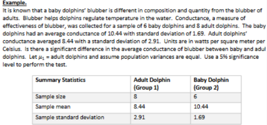
Example: Answer question, EQUAL VARIANCES ASSUMED (solve for BOTH CV and P value)

• **need to determine the test being conducted and what formulas to use based on population variances 

  • “Is there a significant difference in the average conductance” → this indicates that this is a MEAN difference test 

  • “Assume population variances are equal” → this indicates that the f test was performed and failed to reject null 

  • IF THIS IS NOT STATED THEN WE NEED TO PERFORM THE ENTIRE F TEST FIRST!!!

• 1. Hypotheses 

  • Ho: mu1 - mu2 = 0    / mu1=mu2

    • No difference in the average conductance of blubber between baby and adult dolphins

  • Ha: mu1 - mu2 not equal to 0   /  mu1 not equal to mu2

    • There is a difference in the average conductance of blubber between baby and adult dolphins

    • This means we will conduct a TWO TAILED TEST 

• 2. Test statistic 

  • Assume population variance is equal; use specific formula

  • First need to calculate pooled sample variance:

    • sp^2  = [(8-1)(2.91^2) + (6-1)(1.69^2)]/(8+6-2) = 6.12977 = POOLED VARIANCE

      • We square root s because we are GIVEN SD, but REMEMBER that at times will be given variance so will not need to square the values 

      • A way to check that pooled variance makes sense, is to compare to the 2 sample variances, it must be between them since it is an average of them

  • T test statistic = (8.44-10.44) / ( square root 6.12977 ((1/8)+(1/6))) = -1.49577

• 3. T Critical value 

  • qt(alpha/2, df)

    • alpha/2 : 0.05/2 = 0.025

    • df= 8+6-2 = 12 

    • Lower.tail : NOT NEED TO ADD SINCE TWO TAILED, our distribution is normal, therefore critical values will be symmetric, so will just add plus/minus symbol to the CV 

    • qt(0.025, 12) = +- 2.1788

• 3. P value

  • 2 * pt( t test statistic, df, lower.tail=TRUE) 

    • T test statistic:  -1.49577

    • df= 8+6-2=12

    • Need to include lower.tail because the p value is the TOTAL area of BOTH tails 

    • MUST MULTIPLY BY 2 SINCE TWO TAILED

    • 2* pt ( -1.49577, 12, lower.tail=TRUE) = 0.1605

• 4. Decision/interpretation 

  • Critical value

    • T test statistic:  -1.49577 , our CV is 2.1788 , -1.49 does NOT fall within rejection region, falls in middle of graph somewhere between CVs

    • FAIL to reject null; there is no significant difference in the average conductance 

  • P value 

    • Significance level/alpha = 0.05, the p value is 0.1605, p value > significance level 

    • FAIL to reject null; there is no significant difference in the average conductance

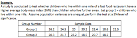
Example: Conduct an F test to prove UNEQUAL variances and T test (solve for F test P value and T test CV)

1. Perform the f test for equality of variances to check that the population variances can be assumed unequal 

• Use R Studio to import data to determine values 

  • Calculating using R: (can do by hand! **remember CANNOT use R on tests)

    • mean(Group1)= 24.2               var(Group1)= 19.003     n=7     

    • mean(Group1)= 20.267      var(Group2)= 2.6747       n=6

• 1. Hypothesis for F TEST

  • Ho: sigma1^2 = sigma2^2

  • Ha: sigma1^2 not equal to sigma2^2 

• 2. Test Statistic for F TEST 

  • F=  (19.0033/2.6747) = 7.1049
    ****NUMERATOR WILL ALWAYS BE THE LARGER SAMPLE VARIANCE, VALUE ALWAYS > 1

• 3. P value 

  • P value

    • 2* pf(7.104933, 6, 5, lower.tail=FALSE) = 0.04814

• 4. Decision/Interpretation 

  • Significance level of 0.05, p value is less than that, therefore we REJECT the null, population variances are UNEQUAL!

2. NOW we can conduct our t test for difference in population means 

• 1. Hypotheses for T test means

  • Ho: mu1 = mu2    / mu1 - mu2= 0

  • Ha: mu1 > mu2    /  mu1 - mu2 > 0

• 2. Test Statistic 

  • V1= (19.003/7)= 2.715

  • V2= (2.6747/6)=0.4458

  • t= (24.2-20.2667 ) / square root [(2.715) + (0.4458)] →

    • (3.933)/ square root (3.1605) = 2.2125

  • df= [(2.715) + (0.4458)]² / [(2.715² /6) + (0.4458² /5)]=

    • [9.989] / [(1.2283) + ( 0.0397)]=  7.8774 → ALWAYS ROUND DOWN → DF IS 7 FOR THIS STUDY 

    • **we need df for the next step 

• 3.T Critical value  

  • T Critical value 

    • ONE TAILED = alpha, TWO TAILED= alpha/2

    • LOWER TAIL FALSE FOR POSITIVE CV (ie for upper tail) and TRUE FOR NEGATIVE CV (ie for lower tail) 

    • qt(alpha, df, lower.tail)

    • qt(0.05, 7, lower.tail=FALSE) = 1.8945
      
      

• 4. Decision/Interpretation 

  • T test statistic is 2.2125, it FALLS in the upper rejection region when comparing to upper CV of 1.895

  • Reject Ho, there is evidence that children who living within one mile of fast food have higher average BMI than those that live further away 

Summary: 

• For independent samples (comparing 2 independent groups)

1. Perform F test to determine if variances are assumed equal/unequal
   ****if problem states whether (un)equal, do not have to perform F test

2. Then, perform T test for difference in population means
   ****assuming equal variances use POOLED formula (df=n1+n2 -2)
   ****assuming unequal variances use the UNPOOLED formula (long tedious df) 

ANOVA Definitions

• Experimental design: plan to test hypothesis where the researcher can control or manipulate 1+ variables 

• Independent variable: variable manipulated by researcher

  • Has 2+ treatments (treatment variable)

• Dependent variable: response variable based on levels from independent, what is being measured

Determine the Independent, Dependent, and # of treatments variables

• Dependent variable: Hunger rating/level, ate that snack then asked to rate how hungry they were after that snack (what each of the above values represent)

• Independent variable: type of snack 

  • 3 treatments; healthy, tasty, no snack 

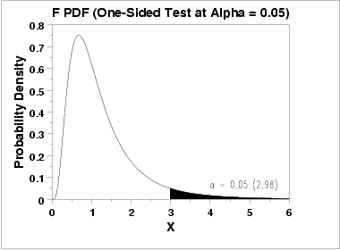
F Distribution Properties

• Right skewed distribution 

• Provides an area (probability) of alpha in the upper tail of the distribution when finding a critical value 

  • Tells us that when we perform an ANOVA, only ONE rejection region, ALWAYS the UPPER TAIL→ no such thing as two tailed when performing ANOVA specifically!!!!!

• Still varies by 2 degrees of freedom 

  • Numerator: df1: k-1

  • Denominator: df2: N-k

ANOVA Properties/Assumptions

• Goal: ANOVA looks at the ratio between group variation to the within group variation to test multiple population means (has to be 3+ means) 

• QUANTITATIVE DATA!!! (analyzing means)

• Between Group variation (treatment group variation)

• Within group variation (error group variation) → variability of one group compared to its mean

Assumptions in ONE WAY ANOVA

• Each of the k population distributions is normal

  • **k= # of populations comparing, # of treatments, # of groups 

• Population SDs for each k distributions are equal (sigma1=sigma2=sigmak)

• K random samples are selected independently from the populations (different samples from different populations)

**overalls still a hypothesis test so has the 4 steps BUT expanded because multiple means 

ANOVA: Step 1

• 1. Hypotheses

  • Null: no difference among all k population means 

    • mu1=mu2=muk

  • Alternative: 

    • Not all population means are equal 

    • At least one (or two) population means are different 

  **both mean the same thing, just different ways to suggest something is different, we aren't actually going to know what is different at this point, must use a FOLLOW UP test to determine which one is 

***Ha CANNOT be written as Ha: mu1 not equal mu2 not equal muk → states that all are unequal which is incorrect. →we do not have notation for this hypothesis so always statement 

ANOVA: Step 2

2.Test Statistic 

• F TEST!!

  • Ratio of 2 variance estimates 

  • MsTr: variance estimate of between (treatment) group variation 

  • MSE: variance estimate of within (error) group variation 

**will need to calculate both of these variances 

ANOVA: Step 2a (ANOVA TABLE)

• The ANOVA table is the tool we use to calculate 

• WE WILL ALWAYS use this table when calculating ANOVA

• All of these steps are to get to that F Ratio (test statistic), summarizes each step used to get to that f test statistic (keeps all of the steps nice and structured 

**if dont have sample mean and variance of each group given in problem, we need to CALCULATE FOR THEM!!!

• F distribution so we still need 2 degrees of freedom 

• k= number of groups, populations, treatments, etc. 

• N= overall sample size for the study 

ANOVA Step 3

3. Critical Value/ p value 

• F Critical value

  • qf (alpha, df1:k-1, df2:N-k, lower.tail=FALSE)

  • **always upper tail rejection region, so alpha and FALSE)

• P value

  • pf (f test statistic, df1, df2, lower.tail=FALSE)

  • Now the f test statistic begins the point of rejection

ANOVA: Step 4

4. Decision/Interpretation 

• F Critical value

  • IF F ratio is greater than the F critical value (rejection region) then we reject the null hypothesis, otherwise fail to reject 

EXAMPLE: Conduct an ANOVA test

**note: a dash- signifies repeating values (REMEMBER TO USE AT LEAST 6 DECIMAL PLACES)

• K=3 (3 different treatments/groups)

1.Hypothesis

• Null: Ho: mu1=mu2=mu3 → no difference in mean hunger ratings between healthy, tasty, and no snack groups 

• Alternative: Ha: not all population mean hunger ratings are equal

2. F test statistic

ANOVA TABLE

Source of variation	Sum of Squares	df	Mean sum of squares	F ratio
Treatment (between)	(SSTr)  16.2-	(k-1)     2	(MSTr)   8.1-	3.859
Error (within)	(SSE)    50.4-	(N-k)    24	(MSE)  2.1018
Total	(SSTo: SStr+SSE)            66.6-	(N-1)   26

• SSTr: sum of ni(x-bar i - x-barbar)^2 

  • X-bar 1= 5.2-    x-bar 2=3.3-   x=bar 3=4.1-   x-barbar= (add every observation)/(total observations-27)= 4.2-

  •   *****(ALSO because sample sizes are equal can average the sample sizes BUT ONLY WHEN SAMPLE SIZES EQUAL!!) 

  • Do that for each group, in this case there will be 3 being added 

  • SSTr: 9(5.22-4.2-)^2 + 9(3.33-4.2-)^2  + 9(4.11-4.2-)^2 =  16.2-

• SSE: sum of (n1-1)s1^2 

  • ***REMEMBER s^2 REPRESENTS VARIANCE – SINCE we’re given variance already we do not have to square the data, but if given sd we DO have to square it 

  • SSE: (9-1)(2.4-) + (9-1)(2.5) + (9-1)(1.3611111) =  50.4-

• SSTo: 50.4- + 16.2- = 66.6-

• Df: k-1: (3-1)=2   N-k: (27-3)=24   N-1: (27-1)=26

• MSTr: SSTr/k-1 

  • (16.2-)/(2) = 8.1-

• MSE: SSE/N-k

  • (50.4-)/(24) = 2.1018

• F ratio (test statistic): MSTr/MSE : (8.1-)/(2.1028) = 3.859

3.Critical Value/P value

• F critical value 

  • qf(0.05,2,24,lower.tail=FALSE) :   3.403

• P value

  •  pf(3.859031,2,24,lower.tail=FALSE) = 0.035
    
    

4.Decision/Interpretation 

• F critical value:

  • Our f test statistic of 3.85 is greater than the f critical value of 3.40 so we REJECT our null hypothesis, not all population mean hunger ratings are equal 

• P value 

  • The p value of 0.035 is less than the significance level of 0.05, so we REJECT our null hypothesis, not all population mean hunger ratings are equal 

LSD Procedure: comparison of pairs of groups in an ANOVA

• THESE TYPES OF PROCEDURES WILL ALWAYS FOLLOW UP ANOVA TEST 

• ***IF PROVEN that there IS a difference in population means (REJECT the null) then we MUST conduct a procedure to determine which of the means are different!!!! ((*****if fail to reject, then we DO NOT need to conduct these procedures since there is no difference in means)

Fishers Least Significant Difference (LSD) 

• Allows us to test if the means of any two populations are significantly different 

• Performed ONLY after a one-way analysis of variance (ANOVA) 

• Consider the ANOVA hypotheses: 

  • Ho: mu1=mu2=mu3=muk

  • Ha: not all of the population means are equal 

• We want to determine which of these pairs of means are different and causing us to reject the null

LSD Procedure

• Will be conducted for every pair of means in the study (AKA: pairwise comparison) 

• How many pairwise comparisons are there? 

  • [K(K-1)] /2    where k= number of populations 

  
  

  • ex) k=3 → [3(3-1)]/2 = 3 → this is telling us that there are 3 pairs that we need to test, meaning we perform this test 3 times!

  
  

  • The more groups we are comparing, the more pairs we are testing/conducting the procedure on!! 

• This is a T TEST, a hypothesis test, so it will follow our 4 step procedure!!! ((just for every single mean pair))

LSD: Step 1

1.Hypothesis 

• Ends up looking like a two sample test 

• Null: Ho: mui = muj

  • (i and j just represents which groups we are testing, either group 1 and group3, etc.) 

• Alternative: Ha: mui not equal to muj 

  • ALWAYS TWO TAILED, since we are just testing if there is a significant difference 

• Additional hypotheses for every pairwise comparisons

• ex) k=3 → 3 means: Ho: mu1 = mu2, mu1 =mu3, mu2 = mu3 , etc. etc.  which means 3 different hypotheses

**whichever group is written first in the question is group 1!! (what comes first) 

LSD: Step 2

2. Test Statistic 

• T TEST!

• Since given some values from our previous ANOVA test, USE THEM!!! ((however if not given the values we must calculate them with given data))

  • Same test stat for t tests BUT The amount of variability now comes from the ANOVA table →

    • MSE = Mean Square error from our ANOVA 

    • df= N-k     (Error degrees of freedom from the ANOVA)

    • The BETWEEN source of variation 

LSD: Step 3

3. Critical Value and P value 

• T critical value 

  • qt(alpha/2, df=N-k)  

  • Since two tailed, do not need lower.tail since +-  

  • (T is symmetric curve)

• P value 

  • 2* pt( - t test stat, df=N-k, lower.tail=TRUE)

  • 2* pt(+ t test stat, df=N-k, lower.tail=FALSE)

LSD: Step 4

4. Decision/Interpretation

• T critical value 

  • If t test statistic falls inside either of the rejection regions, the null hypothesis is rejected, otherwise we fail to reject 

• P value 

  • If p value less than or equal to alpha (significance level) reject Ho 

  • If p value greater than alpha (significance level) fail to reject Ho

  • ***ALPHA WILL REMAIN THE SAME FOR LSD PROCEDURE AS IT WAS IN THE ANOVA TEST

EXAMPLE: LSD Procedure ((Use prev ANOVA test for hunger ratings))

Source of variation	Sum of Squares	df	Mean sum of squares	F ratio
Treatment (between)	(SSTr)  16.2-	(k-1)     2	(MSTr)   8.1-	3.859031
Error (within)	(SSE)    50.4-	(N-k)    24	(MSE)  2.101852
Total	(SSTo: SStr+SSE)            66.6-	(N-1)   26

*p value 0.035 < 0.05 → REJECT the null (thus not all population mean hunger ratings are equal)  

→ now that this ANOVA was conducted and we determined that there was some difference in population mean, we now want to know which pairs of means are significantly different, so we conduct the LSD procedure! 

LSD PROCEDURE FOR THE ABOVE ONE WAY ANOVA TEST 

Determine how many pairs/how many times this procedure needs to be conducted

• k=3 → k(k-1)/2 → [3(3-1)]/2 = 3 pairs ←1. Healthy and tasty, 2.Healthy and no snack, 3.tasty and no snack 

1.Hypotheses  (HEALTHY AND TASTY)

• Ho: mu h = mu t 

• Ha: mu h not equal to mu t 

2.Test Statistic (HEALTHY AND TASTY)

• (xbar h - xbar t) / sq root MSE ((1/nh) + (1/nt))

• (5.2222222-3.333333)/ sq root 2.101852 ((1/9)+(1/9)) = 2.763831854

• df=N-k = 24 

3. P value (HEALTHY AND TASTY)

• 2* pt( + t test stat, df, lower.tail=FALSE) 

• 2* pt(2.763854, 24, lower.tail=FALSE) = 0.01079727

4.Decision/Interpretation (HEALTHY AND TASTY)

• Since our p value of 0.01079727 < 0.05, we reject the null that healthy and tasty population means are equal 

• There is a significant difference in the population mean hunger rating between Healthy and tasty groups 

1.Hypotheses  (HEALTHY AND NO SNACK)

• Ho: mu h = mu ns

• Ha: mu h not equal to mu ns

2.Test Statistic (HEALTHY AND NO SNACK)

• (xbar h - xbar ns) / sq root MSE ((1/nh) + (1/n ns))

• (5.2222222-4.111111)/ sq root 2.101852 ((1/9)+(1/9)) = 1.6257834

3. P value (HEALTHY AND NO SNACK)

• 2*pt(1.6257834, 24, lower.tail=FALSE) =  0.117078

4.Decision/Interpretation (HEALTHY AND NO SNACK)

• Since our p value of 0.117078 is greater than our significance level of 0.05, we fail to reject the null

• There is no difference between the population mean hunger rating between healthy and no snack groups 

1.Hypotheses  (TASTY AND NO SNACK)

• Ho: mu t = mu ns

• Ha: mu t not equal to mu ns

2.Test Statistic (TASTY AND NO SNACK)

• (xbar t - xbar ns) / sq root MSE ((1/nh) + (1/n ns))

• (3.3333333-4.111111)/ sq root 2.101852 ((1/9)+(1/9)) = -1.138048375

3. Critical value (TASTY AND NO SNACK)

• qt(alpha/2, df) 

• qt(0.025, 24) = +- 2.063899

4.Decision/Interpretation (TASTY AND NO SNACK)

• Since the test statistic of -1.138048 does not fall below or above the critical value (does not fall in the rejection region) of +-2.063899 , we fail to reject reject the null that healthy and tasty population means are equal 

• There is not a significant difference in the population mean hunger rating between tasty and no snack groups 

Summary of findings/process 

• We ran the ANOVA and rejected the null, thus we had to perform the LSD procedure. We proved that the healthy and tasty are significantly different. (these were the two groups causing us to reject the null in ANOVA, to get the specific values we had to conduct the LSD procedure). The rest of the population means were not significantly different.