Sampling

Random Samples

• Deterministic Sample:

  • Sampling Scheme doesn’t involve chance

• Random Sample:

  • Before the sample is drawn, you have to know the selection probability of every group of people in the population

  • Not all individuals/ groups have to have equal chance of being selected

Simple Random Sample

A random sample in which:

• every individual in the population has an equal chance of being selected

• individuals are not replaced in the population before the next is drawn

• selecting one individual doesn’t affect the probability of selecting another individuals

Sample of Convenience

• example: sample consists of whoever walks by

• just because you think you’re sampling “randomly”, doesn’t mean you gave a random sample

• if you can’t figure out ahead of time

  • what’s the population

  • what’s the chance of selection, for each group in the population

    • then you don’t have a random sample

Probability Distribution

• random quantity with various possible values

• “Probability distribution”

  • all the possible values of the quantity

  • the probability of each of these values

Empirical distribution

• “Empirical”: based on observations

• Observations can be from repetitions of an experiment

• “Empirical Distribution”

  • all observed unique values

  • the proportion of times each value appears

Law of Averages/ law of large Numbers

if a chance experiment is repeated many times, independently and under the same conditions, then the proportion of times than an event occurs gets closer to the theoretical probability of the event

As you increase the number of rolls of a die, the proportion of times you see the face with firve get closer to 1/6

Empirical distribution of a Sample

if the sample size is large

then the empirical distribution of a random sample with replacement

resembles the distribution of the population

with high probability

A statistic

Instead of always looking at histograms, sometimes we just want to summarize the histogram with a single number

Inference

• Statistical Inference:

  • Making conclusions based on data in random sample

  • Ex: use the data to guess the value of an unknown (fixed) number create an estimate of the unknown quantity (depends on the random sample)

Parameter

A number associated with the population

Statistic

A number calculated from the sample

*A Statistic can be used as an estimate of a parameter

---

Probability Distribution of a Statistic

• Values of a statistic vary because random samples vary

• “Sampling distribution” or “probability distribution” of the statistic:

  • All possible values of the statistic,

  • and all the corresponding probabilities

• Can be hard to calculate

  • Either have to do the math

  • Or have to generate all possible samples and calculate the statistic based on each sample

Empirical Distribution of a Statistic

• Empirical distribution of the statistic:

  • Based on simulated values of the statistic

  • Consists of all the observed values of the statistic,

  • and the proportion of times each value appeared

• Good approximation to the probability distribution of the statistic 

  • if the number of repetitions in the simulation is large

Simulating Statistic (ex: United)

1. Define function

def sample_median (size):

return np.median(united.sample(size).column(‘Delay’))

sample_median = make_array()

for i in np. arange(1000):

new_median = sample_median(10)

sample_median = np.append(sample_medians, new_median)

Probability Sample

is one for which it is possible to calculate, before the sample is drawn, the chance with which any subject of elements will enter the sample

In a probability sample, all elements need nt have the same chance of being chosen

Simple Random Sample

is a sample drawn at random without replacement. Sampled individuals are not replaced in the population before the next individual is drawn.

to use np.random.choice for simple random sampling, you must include the argument replace = false

Convenience Samples 

If you stand at a street corner and take as your sample the first ten people who pass by, you might think you’re sampling at random because you didn’t choose who walked by.

But it’s not a random sample – it’s a sample of convenience.

You didn’t know ahead of time the probability of each person entering the sample; perhaps you hadn’t even specified exactly who was in the population.

Empirical Distribution

The word “Empirical” means “observed”. Empirical distribution are distributions of observed data, such as data in random sample

A Probability Distribution

The histogram helps us visualize the fact that every face appears with probability 1/6. We say that the histogram shows the distribution over all the possible faced. Since all the bars represent the same percent change, the distribution is called uniform on the integers 1 through 6.

variables who’s successive values are separated by the same fixed amount, such as the value on rolls of a dies (successive value separated 1), fall into a class of variables that are called discrete.

the histogram is called a discrete histogram. its bins are specified by the array die_bins and ensure that each bar is centered over the corresponding integer value

The probability of each face is 1/6, which is 16.67% when rounded to two decimal places. The width of each bin is 1 unit. So the height of each bar is 16.67% per unit

*Theoretical probability of each face —- “probability distribution” and not based on observed data

Table menthod for random sample with replacement

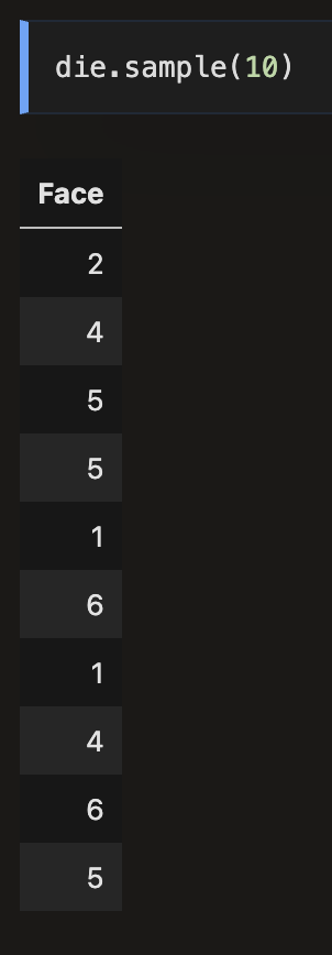
The table method Sample draws at random with replacement from the rows of a table.

Its argument is the sample size, and it returns a table consisting of the rows that were selected

Optional argument:

with_replacement = False — specifies that the sample should be drawn without replacement. But that does not apply to rolling a die

ex: die.sample(10)

Law of Averages

if a chance experiment is repeated independently and under identical conditions, then, in the long run, the proportion of times that an event occurs gets closer and closer to the theoretical probability of an event

Here “independently and under identical conditions” means that every repetition is performed in the same way regardless of the results of all the other repetitions.

Under these conditions, the law above implies that if the chance experiment is repeated a large number of times then the proportion of times that an event occurs is very likely to be close to the theoretical probability of the event.

Converfe of the Empirical Histogram of the Sample

For a large random sample, the empirical histogram of the sample resembles the histogram of the population, with high probability

The idea is that since a large random sample is likely to resemble the population from which it is drawn, quantities computed from the value in the sample are likely to be close to the corresponding quantities in the population

Parameter

Frequently, we are interested in numerical quantities associated with a population.

• in a population of voters, what percentage will vote for candidate A

• In a population of Facebook users, what is the largest number of Facebook friends that user has

• In a population of United flights, what is the median departure delay

Numerical quantities associated with a population are called parameters.

ex: for the population of flights in united, we know the value of the parameter “median delay”

Statistic

In many situations, we will be interested in figuring out the value of an unknown parameter. For this we will rely on data from a large random sample draw from the population

*A statistic is any number computed using the data in a sample. The sample median, therefore is a statistic

The statistic could have different. A fundamental consideration is using any statistic based on a random sample is that the sample could have come out differently, and therefore the statistic could have come out differently too

Just how different could the statistic have been?

One way to answer this is to simulate the statistic many times and note the values. A histogram of those values will tell us bout the distribution of the statistic

Simulating a Statistic

Overview: We will simulate the sample median using the steps we setup in an earlier chapter when we started studying simulation. You can replace the sample size of 1000 by any other sample size, and the sample median by any other statstic

Step 1: Decide which statistic to simulate. We have already decided that: we are going to simulate the median of a random sample of size 1000 drawmn from the population of flight delays

Step 2: Define a function that returns one simulated value of the statistic. Draw a random sample of size 1000 and compute the median of the sample.

def random_sample_median():

return np.median(united.sample(1000).column(‘Delay’))

Step 3: Decide how many simulated values to generate. Lets do 5,000 repetitions

Step 4: use a for loop to generate an array of simulated values. As usual, we will start by creating an empty array in which to collect our results. We will then set up a for loop for generating all the simulated values. the body of the loop will consist of generating one simulated values of the sample median , and appending it to our collection array

medians = make_array()

for i in np.arange (5000)

median = np.append (medians, random_sample())

Visualization

Table:

simulated_median = Table().with_column(‘Sample Median’, median)

Histogram:

simulates_medians.hist(bins = np.arange(0.5,5,1))

you can see that the sample median is very likely to be about 2, which was the value of the population median. Since samples of 1000 flight delays are likely to resemble the population of delays, it is not surprising that the median delays of those samples shelf be closer to the median delay in the population

Simple Random Sample

sample at random with out replacement (with_replacement = False)

If you are sampling from a population of individuals whose data are represented in rows of a table, use

use the table method: sample

If you are sampling from a population of individuals whose data are represented as an array, use

use: np.random.choice

Default: with replacement

#the faces of a die, as an array

faces

array (1,2,3,4,5,6])

#7 rolls of the die

np.random.choice(faces,7)

array([4,1,6,3,5,4,6])

The argument replace = False allows you yo get a simple random sample, that is, a sample drawn at random without replacement

Sampling from a Categorical Distribution

Sometimes we are interested in a categorical attribute of our sampled individuals. For example, we might be looking at whether a coin lands heads or Tails. Or we might be interested in the political parties of randomly selected voters

In such cases, we frequently need the proportions of sample voters in the different categories

Sample_proportions

It is tailored for sampling at random with replacement from a categorical distribution and returns the proportions of sampled elements in each category.

The sample_proportions functions function takes two arguments:

• the sample size

• the distribution of the categories in the population, as a list or array of proporotions that add up to 1

It returns an array containing the distribution of the categories in a random sample of the given size taken from the population. That’s an array consisting of the sample proportions in all the different categories, in the same order in which they appeared in the population distribution.

Example using Sample_proportions

For example, suppose each plant of a species is red-flowering with chance 25%, pink-flowering with chance 50%, and white-flowering with chance 25%, regardless of the flower colors of all other plants. You can use sample_proportions to see the proportions of the different colors among 300 plants of the species.

# Species distribution of flower colors:
# Proportions are in the order Red, Pink, White
species_proportions = [0.25, 0.5, .25]

sample_size = 300

# Distribution of sample
sample_distribution = sample_proportions(sample_size, species_proportions)
sample_distribution

array([0.24333333, 0.50333333, 0.25333333])

sum(sample_distributions)

1

The categories in species_proportions are in the order Red, Pink, White. That order is preserved by sample_proportions

If you just want the proportion of pink-flowering plants in the sample, you can use item

sample_distribution. item(1)

0.503333333