econ midterm ii
 Call Kai
 Learn
 Practice Test
 Spaced Repetition
 Match
 Flashcards
 Knowt Play
1/90

There's no tags or description
Looks like no tags are added yet.
91 Terms
pigouvian tax
per-unit tax imposed on a market activity that generates a negative externality
how does a pigovian tax work?
without intervention, firms only consider their private marginal costs (PMC) and overproduce
the tax forces firms to internalize the external cost of their production
what should the pigovian tax be equal to?
marginal external cost (MEC)
collusion
an agreement among firms about quantities, prices, or other dimensions of competition
these firms may try to behave collectively like a monopolist and increase their joint profits
cartel
a group of firms that coordinates its behavior in an attempt to exercise market power
what problem do cartels face?
incentive to cheat: once other firms restrict output, an individual member may increase its own profit by producing more
oligopoly
market structure in which a small number of dominant firms control the majority of an industry's production, supply, and pricing
how does oligopoly output relate to a monopolist’s?
total output is greater than monopoly output
how does oligopoly output relate to a competitive’s?
total output is less than competitive output
how does oligopoly market price relate to a monopolist’s?
market price is lower than the monopoly price
how does oligopoly market price relate to the marginal cost?
market price is higher than marginal cost
quantity of monopoly, oligopoly, and competitive
Qm < Qo < Qc
price of monopoly, oligopoly, and competitive
Pm < Po < Pc = marginal cost
as the number of sellers in an oligopoly increases…
the market becomes more competitive
price approaches marginal cost
total output approaches the socially efficient quantity
(moves towards the competitive outcome)
nash equilibrium
the end result of a prisoner’s dilemma where each player is choosing their best response to the strategies chosen by the other players
no player can improve their payoff by changing their strategy alone
prisoner’s dilemma
a foundational game theory concept showing how rational choices made by individuals in self-interest lead to a worse outcome for the group
how does the prisoner’s dilemma explain why collusion can be difficult to sustain?
incentive to cheat: an individual firm can increase its own profit by secretly producing more; every firm faces this same incentive to cheat
when is a good rival?
if one person’s use reduces the amount available to others
(example: cup of coffee)
when is a good excludable?
if nonpayers can be prevented from using it
(example: a movie ticket)
private goods
rival and excludable
club goods
excludable and nonrival
common resources
nonexcludable and rival
public goods
nonexcludable and nonrival
finding market demand for private goods
horizontal summation: adding quantities demanded by individuals at each price
finding market demand for public goods
vertical summation: add individual marginal benefits (or WTP) at each quantity
social marginal benefit formula (SMB(Q)) of a public good
MBA(Q) + MBB(Q)
socially optimal quantity (Q*) of a public good
SMB(Q*) = MC(Q*)
the core problem with majority voting
counts people, not the strength of their WTP
revealed preference
valuation methods that infer people’s WTP by observing their actual behavior and real-world choices in related markets
example: to valuate travel cost, observe actual trips taken and expenditures (including opportunity cost of travel time)
stated preference
survey-based valuation methods that directly ask people about hypothetical policies, chances, or bundles to elicit their stated WTP
revealed preference vs. stated preference
revealed preferences use observed behavior; stated preferences capture nonuse values that behavior may not reveal
criticisms of stated preferences
hypothetical bias
WTP vs WTA gap
unformed preferences & survey framing
scope insensitivity (people fail to scale their financial valuation of a problem in proportion to its actual size or magnitude)
adding-up inconsistency
hedonic property values
a revealed preference method that infers WTP for environmental quality (like cleaner air, less noise, or nearby open space) by comparing housing prices while controlling for other home and neighborhood characteristics (size, location, schools)
hedonic wages
a revealed preference method that infers the compensation workers require for greater workplace risk by comparing wages across jobs while controlling for worker and job characteristics (such as skills and working conditions)
what is the main empirical caution when using hedonic property or wage methods?
correlation does not equal causation
if confounding factors (like environmental amenities or job risks) aren’t controlled for, the estimated WTP will be biased
value of a statistical life (VSL)
WTP for a small mortality-risk reduction, scaled to one expected death avoided
VSL formula
WTP per person/risk reduction per person
where does demand come from?
consumers maximizing satisfaction subject to budget constraint

budget graph interpretation: on the line
all income spent

budget graph interpretation: inside the line (shaded blue)
affordable, money left
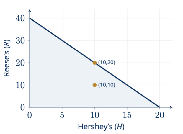
budget graph interpretation: outside the line
not affordable
slope of the budget line
opportunity cost
what happens to the budget line when income changes?
fall in income: budget line shifts inward in parallel
rise in income: budget line shifts outward in parallel
what happens to the budget line when one price changes?
pivots around the intercept of the good whose price did not change
price rises: intercept moves inward
price falls: intercept moves outward
properties of indifference curves (derived from bundles)
every bundle on the same indifference curve yields equal satisfaction
higher indifference curves mean more satisfaction (if both goods are desirable)
curves cannot intersect (if preferences are consistent)
downward sloping (because giving up one good requires gaining more of the other)
marginal rate of substitution (MRS)
the amount of good Y a consumer is willing to give up for one more unit of good X (holding utility constant)
absolute value of the indifference curve’s slope
diminishing marginal rate of substitution (MRS)
along a typical indifference curve, the more X you already have, the less Y you are willing to give up for another unit of X
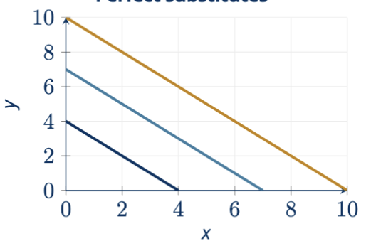
perfect substitutes
constant tradeoff
straight-line indifference curves

perfect complements
fixed proportions
L-shaped indifference curves
graphically finding the optimal bundle
chose the bundle on the budget line that reaches the highest attainable indifference curve (may not be the actual highest curve, as it might lie outside of the budget and be unaffordable)
mathematically finding the optimal bundle
tangency condition: willingness to trade = ability to trade
tangency condition formula
MRSx, y = pricex/pricey
movement along the demand curve
caused only by a change in the good’s own price (px), holding income, other prices, and preferences fixed
shift in demand
caused by a change in income, preferences, or prices of related goods
absorptive capacity
the environment’s ability to absorb pollutants
stock pollutants
persist and accumulate because absorptive capacity is little or absent
(example: carbon dioxide)
fund/flow pollutants
the environment can absorb some of the pollution flow
local, regional, and global pollutants
classified by how far damages extend from the emission source
abatement
the amount of pollution a firm prevents from entering the environment comapred to its unregulated baseline
marginal control cost (MCC)
the additional cost a firm or society incurs to reduce pollution, emissions, or waste by one extra unit
marginal damage (MD)
additional economic or environmental harm caused by one extra unit of an emission, pollutant, or activity
MCC(E*) =
MD(E*)
below E*
extra pollution saves more control cost than the damage it causes
above E*
extra pollution causes more damage than the control cost saved
cost effectiveness
achieving any given pollution reduction target at the lowest possible total cost
efficiency
choosing the socially optimal level of pollution (E*) where marginal cost equals marginal damage AND achieving that reduction cost-effectively
equimarginal principle
to minimize total abatement costs across multiple polluters, the marginal abatement cost (MAC) of the last unit abated must be equal across all firms
MAC1 = MAC2
tradable permits (cap-and-trade)
fix the total quantity of emissions (the cap)
market determines permit price (p)
firms trade permits until MAC = p
who buys vs. sells permits?
high-MAC firms (expensive to clean up) buy permits and abate less
low-MAC firms (cheap to clean up) sell permits and abate more
tax vs. permits
tax fixes the per-unit price
permit fixes total emissions
non-uniformly mixing pollutants
pollutant in which location matters (1 ton emitted upwind of a major city or right upstream of a drinking water intake causes way more damage than 1 ton emitted far away)
(examples: particulate matter, nitrous oxide, smoke from fires)
transfer coefficient (ai)
measures how much pollution concentration at a specific receptor (R; e.g. city or lake) changes when source i emits 1 additional unit
KR (concentration at R) =
background pollution (B) + each source’s emissions weighted by its transfer coefficient (ai)
new equimarginal rule (when location matters)
MAC1/a1 = MAC2/a2
intuition behind new equimarginal rule (when location matters)
a source with a larger transfer coefficient (ai) delivers more improvement at R (specific receptor) per ton abated
equalizing costs per ton of emissions is generally not cost-effective when transfer coefficients differ
coase theorem
if property rights are well defined and bargaining costs (transaction costs) are low, private parties can negotiate to an efficient allocation, regardless of who initially owns the property rights
how should we evaluate public policies?
efficiency and distribution
when is a change a pareto improvement?
at least one person becomes better off
no one becomes worse off
when is a policy a kaldor-hicks improvement?
winners could compensate the losers and still be better off
compensation need not actually occur
net benefits
total benefits = total costs
decision rule
adopt a policy when its social net benefits are positive when accounting for opportunity costs, subject to relevant distributional considerations
opportunity cost of capital
money available today can be invested and earn a return
time preferences
people may value consumption today moret han the same consumption later
changing consumption levels
a future dollar may have different value if future generations are richer or poorer
future value (FVt): interest rates move dollars foward in time
PV(1 + r)t
PV = present value
r = interest rate
prevent value (PV): discounting reverses compounding
FVt / (1 + r)t
what does a more distant payment mean for the present value?
lowers the present value when r>0
what does a higher discount rate mean for the present value?
lowers the present value for a fixed future payment
social discount rate: descriptive approach
look to observed market interest rates and returns to infer how people trade off consumption today against consumption later
social discount rate: prescriptive approach
use ethical judgments and economic reasoning to determine how society ought to value future welfare
ramsey formula
r = p + ng
p = pure rate of time preference
n = elasticity of marginal utility
g = growth rate of consumption per person