unit 2 probability

0.76 Morning or Afternoon

given P(morning) = 0.32 and P(afternoon) = 0.44.

Each customer has exact one caegory, so the events are mutually exclusive.

P(Aor B) = P(A) + P(B)

0.32 + 0.44 = 0.76

If the categories cannot occur together, add without subtracting overlap

0.46 Express or Returned

given P(express)= 0.30, P(returned) = 0.24, and P(express and returned) = 0.08

P(A or B) = P(A) +P(B) - P(A and B)

0.30 + 0.24 - 0.08 = 0.46. Subtract 0.08 because the overlapping orders would otherwise be counted twice.

0.18 Complement of renewing

if 82% renew, the complement means do not renew.

P(not A) = 1 - P(A)

1 - 0.82 - 0.18 (18%)

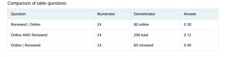
0.30 P(renewed | online)

The vertical bar means given. We are restricted to the 80 online customers. Of those, 24 renewed.

24 / 80 = 0.30.

The condition after the | sets the denominator

Ambiguous

Which is an event?

Experiment: selecting one order

Sample Space: Dine in, carryout, delivery

Delivery is a simple event (one outcome)

Off premise is a compound event.

Both meet the mathematical definition of an event.

Not independent

Independent or dependent?

Given P(renewed) = 0.50 and P(renewed | online) = 0.30

If the events were independent, P(renewed | online) would equal P(renewed). Since 0.30 is not 0.50, the events are independent. This does not prove online shopping causes renewal.

0.12

P(online and renewed)

AND means both conditions must be true. There are 24 such customers out of all 200 customers.

24 / 100 = 0.12

Unlike a conditional probability, there is no specified subgroup after a |.

On time and 3+ days late

Which pair is mutually exclusive?

An individual delivery cannot be both on time and at least three days late.

The other pairs could happen simultaneously.

Ask whether both outcomes could apply to the same observation. If not, they are mutually exclusive

0.40

P(online | renewed)

Now the condition is renewed, so the denominator is all 60 renewed customers. Of those 24, were online.

24 / 60 = 0.40

Notice this differs from P(renewed | online) = 24 / 80 = 0.30

number of returned orders

which variable is discrete?

Discrete: values are counted, commonly 0, 1, 2, 3…(you cannot return 2.5 individual orders)

Continuous: measures such as temperature, package volume, and processing time.

Transaction amounts are generally treated as continuous in basic classes, even though actual payments use cents.

Discrete = count; continuous = measure

Formulas

1.00 Mutually exclusive: 0.40 + 0.60

P(online) = 0.40 and P(in store) = 0.60, with exactly one category. find P(online or in-store)

0.70 Add and subtract pverlap: 0.50 + 0.30 - 0.10

P(A) = 0.50, P(B) = 0.30, P(A and B)= 0.10. find P(online or in-store)

0.25. Complement: 1 - 0.75

75% of packages arrive on time. find P(not on time)

0.40. Divide the 20 renewals by 50 online customers

Of 50 online customers, 20 renewed. find P(renewed | online)

2.00 is the standard error of the sample mean

Why divide by standard error instead of population standard deviation?

Population standard deviation sigma = 8: smaple size n = 16

Compute standard error: Se = sigma / sqrt(n) = 8 / sqrt(16) = 8/4 = 2.00

A sample mean z score measures how far a sample average is from the population mean, in standard errors.

Its denominator is SE, not sigma

Individual value z score uses sigma: sample mean z score uses sigma / sqrt(n)

It decreases

what happens to standard error when n increases?

SE = sigma / sqrt(n).

Holding sigma fixed, a larger n makes sqrt(n) larger, so the quotient get smaller.

Sigma = 8: n = 16 gives SE = 2; n = 64 gives SE = 1

Larger random samples generaly have less variable sample averages

The average processign time for 64 orders was 14 minutes

Identify a sample mean

A sample mean is the average of multiple observations.

Here, 14 minutes summarizes 64 orders.

By contrast, one order took 14 minutes describes a single individual observation.

sample size, number late, and population standard deviation are not sample means.

Look for words like average and mean across a group

=1-NORM.DIST(84,80,2,TRUE)

Probability that a sample mean is at least 84

mean = 80; standard error = 2; target sample mean = 84

Excel syntax: NORM.DIST(x, mean, standard_deviation, TRUE).

TRUE gives the probability at or below x.

Since the question asks for 84 or greater, subtract left-tail probability from 1.

z = (84 - 80) / 2 = 2. P(Z >= 2) is approximately 0.0228, or 2.28%.

-2.00

Calculate the z score of a sample mean

mu =100, sigma = 15, n = 100, sample mean = 97

SE = 15 / sqrt(100) = 15 / 10 =1.5

z = (sample mean - mu ) / SE = (97 - 100) / 1.5 = -3 / 1.5 = -2.00

Negative means the sample average is below the population mean

=1-NORM.DIST(0.35,0.40,0.035,TRUE)

Probability, a sample proportion, is 0.35 or greater

Population proportion pi = 0.40, standard error of sample proportion = 0.0035, target = 0.35

Use NORM.DIST(target, mean, standard_error, TRUE).

Because the question asks 0.35 or greater, subtract the left-tail probability from 1.

z = (0.35 - 0.40) / 0.035 = -1.43\

The probability to the right is approximately 0.9234

0.35 is below the mean of 0.40, so more than half the distribution lies to its right

1.63

Calculate a z score for a sample production

population proportion pi = 0.60, sample proportion p-hate = 0.68, standard error = 0.049

z = (p-hat - pi) / SE = (0.68 - 0.60) / 0.049 = 0.08 / 0.049 = 1.63 (rounded).

Positive means the observed sample proportion is above the population proportion

1.50

Standard error of the sample mean

sigma = 15; n =100

SE= sigma / sqrt(n) = 15 / sqrt(100) = 15 /10 = 1.50

Divide by the square root of n, not n itself

0.022

Standard error of a sample proportion

population proportion pi = 0.25; n = 400

SE = sqrt[pi(1-pi)/n]

sqrt[(0.25)(0.75) / 400] = sqrt(0.00046875) = 0.02165, or 0.022 rounded

Means use sigma / sqrt(n); proportions use sqrt[pi(1-pi)/ n]

more formulas

0.008 describes spread in the original units

Expected value , variance and standard deviation

Expected value E(X) = 1.80, variance = 0.6400, and standard deviation = 0.800.

Expected value (1.80) is the long-run average/center. Variance (0.6400) describes variability in squared units.

Standard deviation (0.800 = square root of 0.6400) measures typical spread in the original units

Mean = center; variance = squared units; standard deviation = original units. An expected value is not guaranteed to occur in any individual trial.

Plan B has higher expected profit and substantially greater variability.

Compare expected profit and risk

expected profit $18,000; standard deviation $12,000.

Plan B: expected profit $24,000; standard deviation $38,000.

Plan B has $6,000 more expected profit, but its standard deviation is $26,000 higher (and more than three times that of Plan A).

Greater standard deviation means a wider range of likely profit outcomes, a common measure of risk.

Avoid answers saying a plan is “automatically better” based on only one statistic. Compare return and risk

1.25

calculate expected value from a probability table

x = 0, 1, 2, 3 and P(x) = 0.20, 0.45, 0.25, 0.10

E(X) = sum of [x × P(x)].

0(0.20) + 1(0.45) + 2(0.25) + 3(0.10) = 0 + 0.45 + 0.50 + 0.30 = 1.25

Multiply each outcome by its own probability, then add. Do NOT divide by the number of outcomes

the long run average approaches about 2.30 calls per hour

Interpret an expected value of 2.30 service calls

2.30 refers to the average over many hours or repeated observations, not the exact number in the next hour.

Individual hours have whole numbers of calls, yet the average can be 2.30

“Expected value” means a theoretical long-run mean, not a prediction guaranteed to happen next

0(0.10) + 1(0.30) + 2(.0.40) + 3(0.20)

Choose the correct expression for E(x)

E(X) = sum of [x × P(x)]. Multiply each possible outcome by its probability.

: 0 + 0.30 + 0.80 + 0.60 = 1.70. Squaring the probabilities (choice D) is not part of the expected-value formula.

For weighted means, bigger probabilities contribute more weight to the average

Each possible value is weighted by its probability

Why expected value resembles a weighted mean

Rather than treating all values equally, expected value multiplies each outcome x by its likelihood P(x). More likely outcomes influence the average more

Probabilities are the weights, and those weights sum to 1 for a valid probability distribution

The probabiities sum to 0.90 rather than 1.00

Recognize an invalid probability distribution

P(x) = 0.25, 0.30, 0.20, 0.15.

: 0.25 + 0.30 + 0.20 + 0.15 = 0.90, not 1.00

Every P(x) must be between 0 and 1 inclusive, AND the probabilities for all outcomes must total exactly 1. This table fails the second requirement.

How much outcomes tedn to vary around the expected value

Interpret standard deviation of 1.55 service calls

Standard deviation describes the typical distance of values from their mean, measured here in service calls.

It is a measure of variability, not a maximum, total probability, or average.

Standard deviation = spread around the mean

Each probability is between 0 and 1 and they sum to 1.

Recognize a valid discrete probability distribution

P(x) = 0.10, 0.30, 0.40, 0.20

0.10 + 0.30 + 0.40 + 0.20 = 1.00; each entry is between 0 and 1.

Always check both conditions. Outcomes may include 0, and probabilities do not need to be equally spaced or strictly greater than 0

even more formulas

Central Limit Theorem

For sufficiently large independent samples with a finite population variance, the sampling distribution of the sample mean is approximately normal even if the original population is not normally distributed

The population itself does not change shape when a larger sample is collected. The CLT concerns the distribution of means across repeated samples.

-0.25

Uniform arrival time

All times in a 12-minute window are equally likely. Probability of landing in a specified 3-minute interval = interval length / total length = 3 / 12 = 0.25 (25%)

With a uniform continuous distribution, probability is proportional to interval length

-15.87%

Interpret an Excel probability

Excel returns 0.1587 as the probability of the requested event.

Multiply by 100: 0.1587 x 100 = 15.87%.

It is not automatically the mean, a z-score, or cutoff

-100

Individual z-score

Given x = 85, population mean = 80, and population standard deviation = 5. z = (x - mean) / SD = (85 - 80) / 5 = +1.00.

This is one standard deviation above the mean.

The value is exactly at the mean.

Interpret z=0

z = (x - mean) / SD. A z-score of zero means x - mean = 0, so x = mean (assuming a positive standard deviation).

=NORM.DIST(95,100,10,TRUE)

Excel lower-tail probability

P(X <= 95), population mean = 100 and population SD = 10.

Excel syntax is NORM.DIST(x, mean, standard_dev, TRUE).

TRUE means cumulative area to the left. Here z = (95 - 100) / 10 = -0.5, so probability is approximately 0.3085

=NORM.DIST(80,70,4,TRUE)-NORM.DIST(60,70,4,TRUE)

Excel probability between values

To find P(60 <= X <= 80), subtract the cumulative probability at the lower bound from the cumulative probability at the upper bound.

P(60 <= X <= 80) = F(80) - F(60).

With mean 70 and SD 4, z cutoffs are +2.5 and -2.5; probability is about 0.9876

The raw value below which about 80% fall

Excel NORM.INV

=NORM.INV(0.80,72,4) gives the 80th percentile of a normal distribution with mean 72 and standard deviation 4. It returns a raw cutoff value, approximately 75.37; 80% of observations fall below this value. NORM.INV is not a probability output

Population mean and population standard deviation.

What mu and sigma represent

mu is the distribution center (population mean).

sigma is population standard deviation, describing spread in the same original units as the variable.

=1-NORM.DIST(84,72,6,TRUE)

Excel upper-tail probability

To calculate P(X >= 84), find the right-tail probability: 1 - cumulative left-tail probability. With mean 72 and SD 6, z = (84 - 72) / 6 = 2.

The upper-tail probability is about 0.0228 (2.28%)

key excel formulas:

Left of x: =NORM.DIST(x,mean,SD,TRUE)

Right of x: =1-NORM.DIST(x,mean,SD,TRUE)

Between a and b: =NORM.DIST(b,mean,SD,TRUE)-NORM.DIST(a,mean,SD,TRUE)

Find a percentile cutoff: =NORM.INV(left_tail_probability,mean,SD)

Individual z-score: (x - mean) / SD

Sample-mean z-score: (sample mean - population mean) / (SD / square root of n

Probability is represented by area over intervals of the density graph.

Which statement best describes probability for a continuous random variable

Step 1: Recognize a continuous random variable. A continuous variable can take any value within an interval, such as package weight, time, or temperature. It is measured rather than counted.

Step 2: Understand how probability works. For a continuous variable, the probability of a range of values equals the area under its probability density curve over that range. The total area under the curve is 1.

Step 3: Remember what happens at one exact value. For any single exact value a, P(X = a) = 0. This does not mean that values cannot occur; it means probability is calculated across intervals, not isolated points. Example: If arrival time is uniform over a 12-minute window, the chance of arriving in a particular 3-minute interval is 3/12 = 0.25. Geometrically, that is 25% of the total area under the density curve

Continuous = area under a density curve. Discrete = add probabilities of specific outcomes