Statistics Exam 1

Population parameter

a number that summarizes a characteristic of the population

Population Parameters Symbols (size N)

• population mean “mu” μ

• population standard deviation “sigma” σ

• population correlation “rho” P

Sample Statistics

a number that summarizes a characteristics of a sample-often estimates an unknown parameter

Sample Statistics Symbols (size n)

• sample mean- x bar X̄

• sample std. dev.- s

• sample correlation- r

Random Sampling Error

different samples naturally include different individuals from population so sample statistics will vary from sample to next and from the true population value by chance

Random Sampling Error Causes

natural, chance variations that happen when you measure a small subset of a population instead of the whole group

How to minimize sampling error

take a LARGE sample from population

Sampling Bias

systematic problem with how sample was collected that causes sample statistic to consistently overestimate/underestimate true population value

Sampling Bias Cause

certain members of a target population more or less likely to be selected than others

How to minimize sampling bias

take a RANDOM sample from population

Samples are a good representation of a population when…

• all choices have equal opportunity to be chosen when randomly selected

• sample is large

Variables

characteristics that vary across sample subjects (columns)

Observations

data collected an individual sample subjects (rows)

Categorical Variables

places individuals into group/category (words, sometimes #s)

Categorical Variables Examples

hair color, favorite movie genre, letter grade on test, level of interest in UT FB

Quantitative Variable

Individual takes on numerical value for which arithmetic operations makes sense (+, -, x, /)

Quantitative Variable Examples

Age, test score, # of concerts attended in past year

Quantitative Variable Scales

• Continuous

• Discrete

Continuous Variable

observations can take on any real numerical value within some range

Continuous Variable Examples

age, test score

Discrete Variable

observations can take on only certain values within some range- typically whole numbers

Discrete Variable Examples

number of concerts attended in past year

Categorical Variable Scales

• Nominal

• Ordinal

Nominal Variable

categories have no inherent order

Ordinal Variable

categories can be organized in some logical order

Nominal Variable Examples

hair color or favorite movie genre

Ordinal Variable Examples

letter grade (A, B, C, D) and level of interest in UT FB (High, Med, Low)

Observational Study

observes individuals and measures variables of interest but does not intervene/apply treatment

Experimental Study

deliberately imposes some treatment on individuals and measures their response

• only establishes causation because they manipulate the independent variable, can randomly assign groups, and control other conditions

Response Variable

outcome variable of the study typically hypothesized to be influenced by one or more explanatory variables in study (dependent variable/outcome variable )

Explanatory Variable

one or more variables are hypothesized to influence response variable (independent variable/predictor variable)

Confounding Variables

an unmeasured variable that masks or distorts the true relationship between the predictor and outcome variables in a study

Can Summarize Categorical Variables Using…

• Frequency (counts)

• Relative Frequency (proportions)

Frequency (counts)

count of all individuals across categories

Relative Frequency (proportions)

how many individuals are in each category compared to the total number of individuals (proportion or %)

Histogram (right-skewed)

Histogram (symmetric)

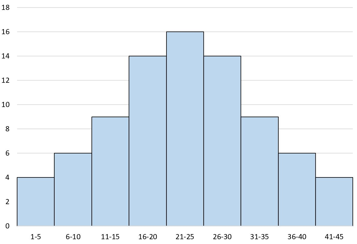
Histogram (left-skewed)

Boxplot (right-skewed)

Boxplot (left-skewed)

Boxplot (no skew)

Measures of Center (Symmetric Distribution)

mean

Measures of Spread (Symmetric Distribution)

standard deviation

Measures of Center (skewed distribution)

Median

Measures of Spread (skewed distribution)

interquartile range (IQR)

Median and IQR are preferred for skewed distributions because…

they are resistant to outliers and extreme values that pull the mean and inflate the standard deviation

Mean and standard deviation are preferred for symmetric distributions because…

the mean accurately represents the center point without being pulled by skewness, and the standard deviation reliably measures the spread of data around that center

Percentiles

• 50th- median

• 25th- lower

• 75th- upper

Stacked Bar Graph

two categorical variables

Side-by-side boxplot

categorical predictor and numeric response

Scatterplots

two quantitative variables

Contingency Table

shows count of the joint (bivariate) relationship between 2 categorical variables

• used to find joint, marginal, and conditional distributions

Joint Distribution

shows how often/what proportion of observations fall into each combination of 2 categorical variables

• calculation: find mean of expected value

Marginal Distribution

shows how data are distributed for 1 variable alone (ignores others)

• found in margins of table in row/column totals

• summing or integrating the joint probabilities or frequencies over all possible values of the other variable

Conditional Distribution

shows the probability distribution of one random variable when the value of another related variable is already known

• calculation: finding the probability distribution of one variable when a specific value or category of another variable is already known

Pearson’s Correlation Coefficient

a statistical number that measures the strength and direction of a linear relationship between two continuous variables

• use when you want to measure the strength and direction of a linear relationship between two continuous, quantitative variables

• 1: Perfect positive relationship (both variables increase together).

• -1: Perfect negative relationship (one variable goes up as the other goes down).

• 0: No linear relationship between the variables

• Calculation: divide how much two variables change together by how much they change individually

Association

two variables move or occur together (correlation)

Causation

one variable directly causes a change in the other

Law of Large Numbers

long-run relative frequency of repeated, independent events eventually produces the true relative frequency as number of trials increase

Mutually Exclusive

outcomes of 2 events cannot occur at the same time

• use addition rule- P(A or B)= P(A) + P(B)

Independent Events

outcome of one event does not affect or change the probability of the outcome of another event

• use multiplication rule- P(A and B)= P(A)P(B)

General Addition Rule

applies to finding prob. of the union of ANY 2 events A and B

• P(A or B)= P(A) + P(B) - P(A and B)

• Events A and B are mutually exclusive if P(A and B)= 0

Joint Probability

the chance both events happen at once

Marginal Probability

chance of a single event occurring, ignoring any other variables

Conditional probability

chance of an event happening given that another specific event has already occurred- “Given that A has happened, what is the probability of B occurring?”

• P(B/A)= P(A and B)/P(A)

General Multiplication Rule

probability of the intersection of ANY 2 events

• P(A and B)= P(A)P(B/A)

• Events A and B are independent if P(B)=P(B/A)

Baye’s Theorem

reverse conditioning event

• Use when you know the probability of the evidence given a cause 𝑃(𝐵|𝐴), but you need the probability of the cause given the evidence 𝑃(𝐴|𝐵)

Law of Total Probability

lets you find the overall probability of an event by breaking the sample space into simpler, non-overlapping scenarios

• use when you need to find the overall probability of an event, but you cannot calculate it directly

Binomial Distribution

use when you are counting the number of successes in a fixed number of independent yes-or-no trials where the chance of success stays the same

Four Conditions of Binomial Model

• Binary outcomes: only 2 possible outcomes

• Independent trials: trial results do not affect each other

• Number of trials is fixed

• Success probability is constant: prob. of success remains the same through all trials

Binomial Formula

Empirical Rule

nearly all data in a normal distribution falls within one, two, or three standard deviations of the mean

• 68-95-99.7 rule

• 68% of data lies within 1 standard deviation (μ ± 1σ) of the mean.

• 95% of data lies within 2 standard deviations (μ ± 2σ) of the mean.

• 99.7% of data lies within 3 standard deviations (μ ± 3σ) of the mean

Converting from Observed (𝑥) to Standardized (𝑧)

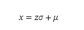
Converting from Standardized (𝑧) to Observed (𝑥)

Variables within Data Frames (RStudio)

When you import a dataset into RStudio, it becomes an object called a data frame. A data frame consists of rows (observations) and columns (variables)

• #See first few rows of the data —> Head(name of dataset)

• To call out a specific variable —> dataset name$variable

Descriptive Statistics (RStudio)

• Measures of center/spread for a numeric variable —> mean(dataset name$variable)</p></li><li><p>Standard Deviation —> sd(dataset name$variable)

• Five Number Summary —> fivenum(dataset name$variable)</p></li><li><p>Frequencies for a categorical variable —> table (dataset name$variable)

Purpose of subsetting in R

extracting specific elements, rows, or columns from a vector data frame or matrix

Logical Expressions

Expression	What it Means
\(>\)   \(<\)	Greater than/less than
\(>=\)   \(<=\)	Greater than or equal to/less than or equal to
\(==\)	Equal to
\(!=\)	Not equal to
&	Logical “and”
\(\mid\)	Logical “or”

Indexing

the location within a variable or data frame, and R uses square brackets [ ] to specify indices

• indexing a variable, you only provide one number

• index a data frame, which is two-dimensional, you need two numbers separated by a comma

- first index for a data frame specifies the row(s) and the second specifies the column(s)

- If you leave one of the indices blank, R will select all rows/columns

Subsetting a Data Frame

subset: pull out specific cases based on some criteria

• after running the above code, a new data frame will appear in your Environment window

R values scatterplot

• r>0 is positive

• r<0 is negative