FINA 4321 Portfolio Management MIDTERM

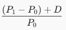
return

measure of how well a security or a portfolio performs

stock holding period return

P0: begin. per. stock price

P1: end of per. stock price

D1: dividends paid (if any) right before the end of the period

income yield

dividends received by the investor (ex. interest earned from the bank)

capital gain or loss

change in security price

Fisher equation

to go from nominal returns to real returns (and vice versa)

• inflation = growth rate in CPI

real return

return adjusted for inflation; shows true purchasing power

• RR of cash is negative if i>0%

nominal return

return at face value before adjusting for inflation

• NR of holding cash = 0% w/ no dividends

expected value

mean of a random variable

• estimated using calculated sample mean based on past returns

stock return

viewed as a random variable b/c its realization is uncertain

variance

avg distance from the mean (units = sq. of original); measure of investment risk

standard deviation

average distance from the mean (units = same as original); measure of investment risk

• sq. root of variance

• interpret: the stock return typically deviates by __ % from the avg return of __ %

covariance

how 2 variables move together; measures direction; scale = infinite

• positive # = move together

• negative # = move opposite

correlation

how 2 variables move together; measures strength and direction; scale = -1 to 1

• positive # = move together

• negative # = move opposite

simple linear regression

best line that describes the relationship between 2 variables

• error term: dist b/w point and regression line

• errors minimized by ordinary least square

coefficient of determination (R2)

how much of the variation in Y is explained by X; scale = 0 to 1

alpha

the intercept of the regression; the value of Y when X is 0

t-stat

t-stat > 1.96 means the coefficient is statistically significant (aka different from 0)

• for alpha or beta

beta

the slope of the regression; on avg, when X increases by 1%, Y increases by (beta)%

returns across various assets

• treasury bills: ST loan to gov; low risk, low returns

• bonds (gov and corp): LT, receive periodic CPNS then principal is paid back at maturity; mid risk, mid returns

Stocks: ownerships to corporations that are entitled to receive cash dividends; high risk, high returns

security returns based on firm characteristics

• size (market cap)

  • small firm = higher TOT risk, higher returns (not higher market risk/beta)

• industry affiliation

• accounting ratios (BTM)

  • value firms have higher returns and risk than growth firms

How security returns behave compared with their risk

Relation between average returns and dispersion (risk) is not trivial (simple/linear)

benefits of diversification

even naive diversification reduces risk considerably (ex. picking stocks randomly)

• downward trend, but the relationship is not monotone (adding a stock does not strictly decrease volatility every single time)

utility function

used to rank and choose among different investment alternatives

• same utility = no preference b/w risky or RF asset

risk aversion

The higher the A, the more the investor dislikes risk

• A>0: risk averse (prefers RF if RP=0); paying for insurance

• A=0: risk neutral

• A<0: risk-loving (prefers risky if RP=0)

• A doesn’t matter if sd=0 (constant returns)

determines which securities an investor selects

risk premium

E(R)-Rf; expected excess return

indifference curve

all the combos of risk and expected return that give an investor the same amount of utility

• one for each level of utility (infinite possibilities)

indifference curve breakdown

• risk averse = steep curve (requires massive return for extra risk)

• risk loving = flatter curve (required minimal return for extra risk)

• higher intercept = higher utility (closer to NW area = highest return, least risk))

risk neutral investor

only cares about expected return and completely ignores risk/volatility (A = 0, U=E(R))

indifferent between investments

investor derives the same utility from both investments

• every point along indifference curve

portfolio

combo of securities indicating the amount invested in each one to balance risk and return

3 rules of portfolio algebra

To characterize the risk and return of ANY portfolio

1. E(R) of a portfolio is the weighted avg of the E(R) of the securities in the portfolio

2. sum of the weights of each security in a portfolio is ALWAYS 1

3. Variance formula for 2 assets

• covariance = 0 if 1 risky and 1 RF (constant return)

capital allocation line

shows all the risk and return combos from a portfolio of 1 risky and 1 RF asset

• slope = sharpe ratio of risky asset

• every portfolio on the same CAL = same Sharpe ratio

buying on margin

borrowing money from a broker to buy stocks

• investor benefits if stock price increases

short selling

Selling something you don’t own

• Investor benefits if stock price decreases

short selling example

borrow a security from a broker and sell it, then buy it back later and return the security

CAL for buying on margin (borrowing)

TOT risk surpasses stock risk

CAL for short selling

only short if Rf > E(R) b/c all earned proceeds are the Rf

sharpe ratio

how much excess return an investor receives for taking on extra risk; measures risk-adjusted return

• slope of the CAL

• interpret: asset earns (SR)% of excess return above the Rf for every 1% of risk

optimal portfolio

proportion you should invest in the risky asset; tangent of the indifference curve and CAL;

• Xs decreases when A or sd increases

• Xs increases when E(R) increases

• Formula derived from maximizing utility, subbing E(Rp) and sd(Rp) values

minimum variance frontier

set of RISKY portfolios with the lowest variance for each level of return

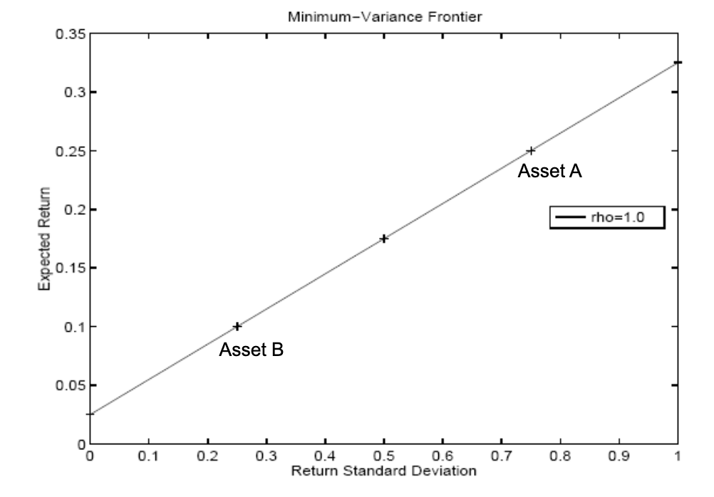
minimum variance frontier for correlation=1

highest risk b/c if one does poorly, so does the other (no buffer)

• like holding one stock

• small gains from diversification

• investment opportunties set will curve slightly left

minumum variance frontier for correlation=-1

lowest risk b/c 2 risky assets move in opposite directions (performance cancels)

• high gains from diversification (lower risk for same level of E(R))

• investment opportunties set will curve sharply left (NW area)

perfectly hedged portfolio

portfolio of risky assets with zero risk; when correlation=-1

minimum variance frontier for correlation=0

efficient frontier

the set of portfolios that have the highest possible expected return for a given level of risk.

minimum variance portfolio

the portfolio of RISKY assets which has the lowest standard deviation

diversification

combining risky securities into a portfolio in order to reduce total portfolio risk

• eliminates firm-specific risk, but not market risk (beta)

Two-Fund Separation Theorem

All portfolios on the Minimum Variance Frontier can be found by combining ANY two distinct portfolios that are also on that frontier

• Useful when constructing a minimum variance frontier with N assets to avoid multivariate optimization and vector algebra

• If portfolios Y and Z lie on the Minimum Variance Frontier, any new portfolio P constructed from them is also on the frontier

systematic and non-systematic risk

because the average covariance between the securities in the NYS is positive, we should not expect to completely eliminate market risk in a large diversified portfolio

• systematic/market risk - interest rate changes, recessions, geopolitical conflicts

• non-systematic/ firm-specific - mismanagement, product failures, labor strikes

optimal risky portfolio (many risky securities and 1 RF asset)

tangency point of the CAL and the efficient frontier; maximum sharpe ratio (slope)

• weight invested is determined by the investor’s risk aversion

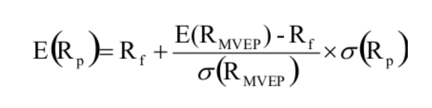
mean variance efficient portfolio (MVEP)

the portfolio of risky assets that has the HIGHEST SHARPE RATIO

• maximizes the reward per unit of risk

optimal CAL

CAL with the maximum sharpe ratio (slope)

• any portfolio on this line is an efficient portfolio

• obtained by combining the risk-free rate with the MVEP

• slope is the sharpe ratio of the MVEP

optimal global portfolio

agents will combine the risk-free asset with the MVEP in different proportions

• everyone chooses the MVEP, but high risk averse investors will invest more on the RF asset and low-risk-averse investors will invest more on the MVEP (and possibly borrow at the risk-free rate)