Fishery exam 2

largemouth bass in peter lake eat all the prey entered in this “cost curve”

• Their diets include everything from Daphnia to warblers, frogs, Snakes, and 7 spp. of mammals!

• no exploitation of this pop, therefore the bass density is very high. that means that competition for food is very intense

calc is the math of dynamics/change

• area under curve is a sum

• time discrete function → dx/dt

allocthonous

food/energy source from outside

autochthonous

food/energy source from within

crayfish - How does a smallmouth forage in an optimal way when crayfish are the prey?

• among preferred prey of small mouth bass

• Crayfish have effective defenses.

• This bass is not foraging optimally! The crayfish is fighting for its life. The bass is losing foraging time

• by coming from behind, the bass is able to stay out of the way and sneak up on the crayfish to successfully capture them

prey capture rate can be increased through learning

chance to learn increases with prey density.

increased skill to attack and capture the prey and/or increased ability to find/detect the prey

functional responses (Holling)

In type I there is a linear relation between prey density and the maximum number of prey killed

in type II the proportion of prey consumed declines monotonically with prey density.

Type III is described by a sigmoid relation in which the proportion of the prey consumed is positively density-dependent over some regions of prey density.

3 ways to describe an ecological concept

• verbally

• graphically

• mathematically

Holling’s disc equation (type II)

• P_e = a’T_sN

• P_e = # of prey eaten per unit time

• a’ = attack rate or search efficiency

• T_s = time spent searching for prey = T_tot - T_hP_e

• T_h = per prey handling time

collapse and failured recovery of northern cod stocks

• the cultivation/decompensation hypothesis

• why haven’t cod recovered

  • we continue to eat them

the cultivation-depensation hypothesis: trophic triangles

the predator pit

a critical intersection point marks where the abundance level above which the rate of production exceeds the rate of predation mortality and the population increases (prey pop achieves breakout) and below which the rate of predation mortality exceeds the rate of production (prey pop collapses into the pit)

models of predator prey dynamics: lotka volterra prey equation

describes the rate of increase of the prey pop

dR/dt = rR - cRP

• cRP = number of prey killed

• R = # prey

• P = # predators

• r = prey’s per capita exponential growth rate

• c = constant expressing efficiency of predation

models of predator prey dynamics: lotka volterra predator equation

describes the rate of increase of the predator pop

• dP/dt = acRP - dP

• acRP = predator recruitment

• P = # predators

• R = # prey

• a = efficiency of conversion of food to growth

• c = constant expressing efficiency of predation

• d = constant related to the death rate of predators

discrete time form of prey equation

R_t+1 = R_t + rR_t - cR_tP_t

discrete time form of predator equation

P_t+1 = P_t + acR_tP_t - dP_t

blue crab females can’t mate until they molted their shell (soft shell crab)

• very vulnerable at this time → males defend the females

• “sponges” under their tail which is the fert eggs

• females migrate to edge of estuary and spawn

recruitment

• the number of individuals that reach a specific stage in the life cycle”

  • eg age 1 or recruitment to the fishery or to a survey gear

• highly variable

  • under the right conditions, a small spawning stock can pull off a huge recruitment

what determines recruitment - match mismatch hypothesis

• cushing 1975

• most larvae starve to death, often at the time of first feeding (after yolk sac used up) → “critical period”\\

• in temperate latitudes, spring phytoplankton bloom followed by zooplankton bloom - timing varies

• spawning time depends on cues like temp and day length - timing varies

• in years in which larval first feeding matches zoop abundance peak, larval survival is high(er)

what determines recruitment - ocean stability hypothesis

• lasker 1981

• patches of food (and particles of all sorts) develop when the ocean is calm

• wind and waves mix the particles over a larger volume

• food aggregations are critical for larval survival as overall food density is low as is their search ability

• but moderate turbulence increases encounter rates at low prey density

• life at low reynolds number

reynolds number Re

• Re = inertial forces/viscous forces = Ud/v

• U = velocity: of an organism (cm/s)

• d = distance: length of an organism, in cm

• v = kinematic viscosity of water, about 0.01 cm2/s

• typical swimming speed for fish is 1 body length/s

• larval herring length at first feeding: 0.9cm

• human swim speed = 2m/s

what determines recruitmen? predation

“bigger is better”

those who grow fastest survive

predation rates are size dependent

bigger is better, but growth has substantial costs

when does dispersal happen

• depends

• clownfish - larval stage

• striped marlin - adult stage

how far do fish disperse

depends on pelagic larval duration (for larvae)

implications of dispersal for management

• limited control over dynamics - substantial harvest or other mortality may occur beyond your jurisdiction

• difficult to tease apart distribution changes from abundance changes (maybe the fish have just moved beyond reach of the survey or fishery)

• so where possible,, stock assessment and management should happen at the level of the unit stock - stock = population

  • great bay striped bass vs sacramento river winter-run chinook

stock identification

• tagging

• genetics

• natural and unnatural chemical tags

  • natural stable isotopes in tissues, trace metals in otoliths

  • contaminants - only when the contaminant has a known source location (ex Fukushima and pacific bluefin tuna)

• parasites

  • The ideal tag parasite is a parasite that has significantly different levels of infection among localities which persist for a long period (a permanent parasite), that is easily detected and identified, and that does not cause serious damage to the host

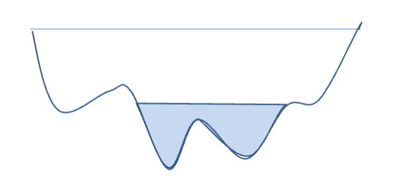
density dependent habitat use

• ideal free distribution - realized suitability is equal in all habitats

• basin model - topographically depicts resource availability

  • low energy dip → gaining highest return on investment

  • fish are in the best habitat until the pop level reaches a point where they spill into the other habitats

• can lead to hyperstable CPUE - CPUE stays high even as the pop declines

climate induced range shifts

many expect northern shift but can also see shift south/down slope to deeper waters

bioenergetics

a conceptual and quantitative approach to understanding fish growth and condition

fish growth - why do we care

• envi indicator, effects fish survival, fisheries management, repro fitness, indicator of “success,” highly variable

fish growth - high variability

• conditions (temp, DO…)

• prey availability

• time

• region

factors affecting fish growth

• diet

  • lake trout that feed on plankton grow more slowly than fish eaters/piscivores

what factors affect lake trout diet

• prey availability

  • some lakes have forage fish, others not

• abundance of forage fish varies (among lakes, among years)

stunting

• slow growth rate = small size at age

• reasons for stunting

  • limited food

  • high densities of fish

• effects on repro? early or late?

fish condition

• measure of fish “chunkiness”

• standardized weight

  • plot length - wright relationship for fish in pop

  • fit regression equation

  • solve equation for common sized fish

allometry

weight-length relationship

predicting growth using bioenergetics

growth - f(consumption, temperature)

Fish Growth: a bioenergetic perspective

• biomass change = consumption - (energy costs + wastes)

  • deltaB = C - (R+ SDA + G + E + F)

• energy input → C = consumption; food/energy input

• energy costs → things fish do

  • R = respiration (metabolism; activity)

  • SDA = specific dynamic action (digestion)

  • G = gonad growth (repro)

  • F = egestion (feces; undigested waste)

  • U = excretion (urine)

consumption as a function of temperature

• temperature = measure of kinetic energy

• temperature affects on metabolism (R)

  • metabolic constaraints = R * f(T)

% consumption as a function of DO

• energy input = C * f(DO)

• f(DO) = multiplier on consumption

  • f(DO) = 1 at max %DO

  • f(DO) < 1 with decreasing %DO

  • f(DO) → 0 in anoxic conditions

DO saturation declines with temperature

DO - amount of oxygen in water

dissolution is function of temp

hotter = less DO

temp-DO interaction

energy input = C * f(DO,T)

seasonal cohorts - ex: Anchoa mitchilli (bay anchovy) in Chesapeake Bay

• bay anchovy synchronous batch spawner june-sept

  • cohorts about 2.5 weeks separated

• life histories depend on time of year

  • spawn timing

  • conditions

  • prey availability

• energy budget function of temp

  • assume: max consumption, weight constant

  • no digestion (large egestion) → energy input and action = 0

• conditions are month dependent

  • how do initial conditions differ among cohorts

  • what conditions differ over months? how?

• what are consequences to cohorts

  • which cohort grows fastest? when?

  • which cohort grows largest?

  • how will cohort sizes differ after year 2

Von Bertalanffy growth model (VBGM)

• VGBM estimates size-at-age

• L_a = L_inf * [1 - e^{(-k* (a-t0))}] = length at age a

• Linf = mean length (cm) of oldest individuals

• k - growth coesfficient

• a = age (yr)

• t0 = length at age 0 (yint)

• if t0 = 0 simply to: L = L_inf * (1- e^-k*a)

how will climate change impact growth of salmonids in mongolia

Lenok and grayling will either grow slower or need to eat a lot more to maintain their historic growth rates… Probably both

R²

the measure of spread around a line/curve

stock assessment in principle

the use of various statistical and mathematical calculations to make quantitative predictions about the reactions of fish populations to alternative management choices

• making predictions

• fisheries management vs stock assessment

• pop dynamics vs stock assessment

stock assessments in practice

• stock assessments aren’t done until there is a problem

• fishermen’s livelihoods and the sustainability of fisheries depends on decisions that are informed by stock assessments

• everything is measured with error, some measurements are biased

• reducing fishing effort is very difficult

• despite uncertainty, decisions must be made

graphical methods and max sustainable yield (MSY)

• N = size of pop

• t = time

• t-1 = previous time measured (N_t-1 = last measured pop size)

• r = pop growth rate

• k = carrying capacity

• as k goes up, the ratio gets smaller if 1-N_t-1 stays the same

• 1-N_t-1 gets smaller as N_t-1 gets bigger (start to lose pop growth as approach k)

• the more fish, the more you catch → eventually reach a max CPUE and then decreases

conceptual framework

• N = pop size

• E = effort

• C = catch

• q = scaler

pop dynamic models (discrete or continuous time)

• exponential N_t = rN_t-1 (discrete time, difference model)

• exponential dN/dt = rn or N_t = N₀e^rt (continuous time, differential equation)

model complexity and numerical vs structural uncertainty → how do you decide how realistic/complex to make the pop model

fit to curve of best fit and adjust

don’t often know what k is

model complexity and numerical vs structural uncertainty → how do you decide how realistic/complex to make the pop model: simulation and assessment

• simulation

  • parameters are known, data is generated

  • used to test assessment models

• assessment

  • parameters are unknown and are estimated by fitting a model to catch, effort, or other timeseries

Simulation model for taimen

• no time series data available

• growth model from literature and few dead fish (otoliths/ear bones)

• mortality from growth model parameters and life history invariants (pauly method)

• carrying capacity from surveys (snorkel and mark recapture) and equilibrium assumption

• project population forward under various fishing mortality scenarios

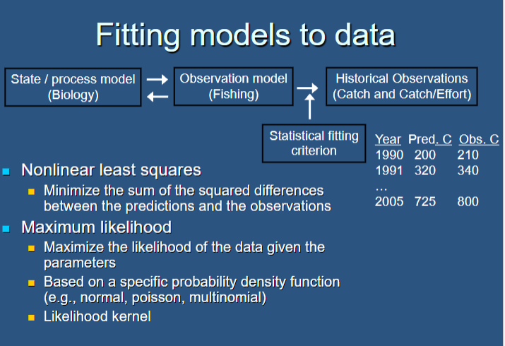
fitting models to data

contrast in catch series

you cannot understand how a stock will respond to exploitation unless the stock has been exploited

adaptive management

• admit uncertainty

• experiment and monitor

fishery independent data

when scientists measure how many fish they catch, not taking into account commercial fisheries (do surveys everywhere, even where there are no fish)

fishery dependent data

take into account data from the fishery/commercial practice

shifting baseline

stock assessment methods typically assume that the catch time series started at virgin biomass

fishermen’s (and manager’s) expectations change over time

error propagation

• N_t = N_t-1 + rN_t-1(1-N_t-1/K)

• k(r) = error

stock recruit relationships - beverton holt

• compensation

• survival increases as SSB declines

• resource limitation (nursey habitat, food, etc)

stock recruit relationship - ricker

• overcompensation

• survival increases rapidly as SSB declines

• survival increase more than compensates for the loss of spawners

• cannibalism, spawning, interference, disease, predator support

  • want to keep SSB where it makes the most fish by taking enough fish where they won’t eat themselves - sustainable yeild

taking too much SSB does not mean the fishery collapses

collapses is when there aren’t enough replacing themselvesr

ricker equation

• R = aSe^-bS

• R = recruitment

• a = scaler

• b = birth rate

• s = spawning stock biomass

B_MSY

the biomass at which MSY is achieved

MSY

number of fish that you want to take out of the pop in order to get the highest # recruits

estimating MSY reference points from your pop model

• analytical solution (schaefer model)

  • MSY = rK/4

  • BMSY = K/2

  • UMSY = r/2

  • r = # recruits

  • k = carrying capacity

• numerical solution

  • Estimate model parameters

  • Simulate a range of different harvest rates and record the long-term average yield.

  • Select the harvest rate that maximizes the long-term average yield and find the associated biomass and catch

UMSY

fishing removal at MSY

yield per recruit

• You can’t control recruitment, but you can change the size/age and intensity of harvest from a cohort

• Harvest too young or too heavily and you’re missing out on growth (growth overfishing)

• Harvest too old/too lightly and many individuals will already have been lost to natural mortality

biomass

number of fish x weight

spawning stock biomass per recruit (recruitment ovrfishing)

Fmax is where you want to fish

F_0.1

fish a little less, catch a little less, but have much less impact on the population

the yield at 10% of the slope at the origin

take 10% of the slope at the origin, then change the y int to raise the slope to be tangent to the curve

selectivity matters

increasing the age at entry into the fisheries results in higher yield

irrespective of the age of entry into the fishery, high yield is generally obtained at intermediated fishing mortality

isopleth

contours

epitaph for MSY

• larkin 1977

• biological complications

  • age of spawners

  • periods of low productivity

  • economic inefficiency

  • estimation problems

target and limit reference points

• MSY is better as a limit reference point than as a target.

• Biomass will still be frequently (approximately half of the time) below BMSY and occasionally well below BMSY

• Blim – the spawning stock biomass below which recruitment is impaired or stock dynamics are unknown

risk of overfishing

• There is always uncertainty in both the estimates of current stock status and in the estimates of reference points

• The acceptable risk of exceeding a threshold reference point is a management, not a scientific, decision

• The role of science is to quantify the risk of exceeding a threshold reference point based on different decisions

OFL - Overfishing limit

the estimated harvest that would result in F>FMSY – determined by the stock assessment

ABC – Acceptable Biological Catch

the OFL minus a buffer for scientific uncertainty based on a stated (or implicit) risk policy

TAC – Total Allowable Catch

the ABC minus a buffer for management uncertainty

Harvest Control Rules

recognize that stock status can change and management should become more precautionary when the stock is in an undesirable state.