Chapter 7 - Understanding Java Performance
 Call Kai
 Learn
 Practice Test
 Spaced Repetition
 Match
 Flashcards
 Knowt Play
1/35

There's no tags or description
Looks like no tags are added yet.
36 Terms
How to think of performance?
Developers often waste time micro-optimizing code (e.g., debating streams versus loops or tweaking method dispatch) when the code itself isn't the problem. In typical systems, bottlenecks usually originate outside application code—in databases, file systems, or networks.
Effective optimization requires measuring what actually impacts the end user—such as average response times and scalability under traffic spikes—rather than optimizing low-level language idioms without profiling first.
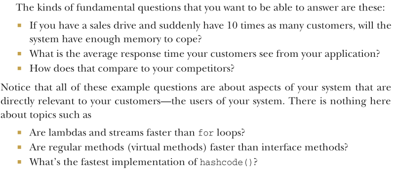
There’s no secret sauce to performance
Modern software systems are complex, meaning performance is an emergent property of the entire system rather than the sum of isolated code snippets. Because of this, reductionist approaches and microbenchmarking rarely help typical application developers identify real bottlenecks.
Effective performance tuning requires moving from guessing to measuring based on real user impact. It is NOT:
A shortcut or "secret sauce"
"Fairy dust" applied at the end of development
A static collection of "tips and tricks"
Relying on generic tips is especially counterproductive on modern JVMs. Without measuring in context, micro-optimizations are often useless, potentially harmful, and quickly made obsolete by ongoing runtime compiler optimizations.
What is Latency?
Latency is the end-to-end time taken to process a single work unit at a given workload.
An often-useful performance measure is the graph showing latency as a function of increasing workload.

What is Throughput?
Throughput is the number of units of work that a system can perform in some time period with given resources.
One commonly quoted number is transactions per second on some reference platform (e.g., a specific brand of server with specified hardware, OS, and software stack).
What is Efficiency?
The efficiency of a system is equal to the throughput divided by the resources used. Efficiency = Throughput / Resources
A system that requires more resources to produce the same throughput is less efficient.
For example, consider comparing two clustering solutions. If solution A requires twice as many servers as solution B for the same throughput, it’s half as efficient.
Remember that resources can also be considered in cost terms—if solution A costs twice as much (or requires twice as many staff to run the production environment) as solution B, then it’s only half as efficient
What is Capacity?
Capacity is the number of work units (such as transactions) that can be in flight through the system at any time.
That is, it’s the amount of simultaneous processing available at a specified latency or throughput.
What is Scalability?
As resources are added to a system, the throughput (or latency) will change. This change in throughput or latency is the scalability of the system
Doubling resources to achieve double the throughput represents ideal linear scaling, but fundamental constraints (like Amdahl's law) make this exceedingly difficult in practice.
You should also note that the scalability of a system depends on a number of factors, and it isn’t constant. A system can scale close to linearly up until some point and then begin to degrade badly. That’s a different kind of performance elbow.
What is Degradation?
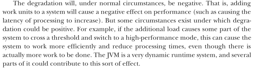
If you add more work units, or clients for network systems, without adding more resources, you’ll typically see a change in the observed latency or throughput. This change is the degradation of the system under additional load.
Setting Clear Goals and Observables Before You Optimize
Many developers, when they approach the task of performance analysis, don’t start with a clear picture of what they want to achieve by doing the analysis. A vague sense that the code “ought to run faster” is often all that developers or managers have when the work begins
To do really effective performance tuning, you should have think about some key areas before beginning any kind of technical work. You should know the following things:
What observable aspects of your code you’re measuring
How to measure those observables
What the goals are for the observables
How you’ll recognize when you’re done with performance tuning
What the maximum acceptable cost is (in terms of developer time invested and additional complexity in the code) for the performance tuning
What not to sacrifice as you optimize
You have to measure. Without measurement of at least one observable, you aren’t doing performance analysis.


Know what you’re measuring
To be a good performance engineer, you should understand terms such as mean, median, mode, variance, percentile, standard deviation, sample size, and normal distribution.
Knowing what you’re measuring and having confidence that your numbers are accurate is the first step. But vague or open-ended objectives don’t often produce good results, and performance tuning is no exception. Instead, your performance goals should be what are sometimes referred to as SMART objectives (for specific, measurable, agreed, relevant, and time-boxed).

What is Sample Size (n)
What it is: The total number of individual measurements collected during a benchmark or observation period.
Why it matters in performance: If you test an API endpoint only 5 times, your results are statistically meaningless—you might get lucky and measure five cache hits, or unlucky and catch one garbage collection pause. A robust sample size (thousands or millions of requests) ensures your observations reflect system behavior rather than random noise.
What is Mean (Average)?
What it is: The sum of all observed values divided by the total count.
Why it matters in performance: Mean response time gives a quick baseline, but it is notoriously deceptive in latency analysis. A single 10-second timeout can drag the mean of ninety-nine 10 ms requests up to roughly 110 ms, hiding the fact that 99% of users had an instant experience.
What is Median (50th Percentile)?
What it is: The middle value when all observations are sorted from lowest to highest.
Why it matters in performance: Unlike the mean, the median is resilient to outliers. If 50% of your requests finish in under 12 ms, the median is 12 ms—regardless of whether the worst request took 50 ms or 50 minutes. It represents the typical experience of an ordinary user.
What is Mode?
What it is: The value that appears most frequently in your dataset.
Why it matters in performance: The mode helps identify recurring, discrete states. For instance, if your latency distribution has two prominent modes (a "bimodal" distribution)—one spike at 5 ms and another at 105 ms—it often signals a clear architectural split: requests hitting an in-memory cache versus requests falling back to a 100 ms database query.
What is Percentile (e.g., p90, p95, p99)
What it is: The threshold below which a given percentage of observations fall.
p90: 90% of requests are faster than this value; 10% are slower.
p99: 99% of requests are faster; only the worst 1% are slower.
Why it matters in performance: This is the industry standard for Service Level Objectives (SLOs). End-to-end user transactions often make dozens of internal sub-requests. If your individual services have a bad p99, a customer will hit that tail latency on almost every complex page load. Tuning the "tail" (p99/p99.9) is where most production stability work happens.
What is Variance?
What it is: A mathematical measure of how spread out the data points are from their mean (the average of squared differences from the mean).
Why it matters in performance: Variance quantifies instability. High variance means your system is jittery and unpredictable; low variance means response times are uniform and steady. Because its units are squared (e.g., ms2), developers rarely quote variance directly, preferring its square root: standard deviation.
What is Standard Deviation?
What it is: The square root of variance. It expresses the average distance of data points from the mean in the same units as the measurement (e.g., milliseconds).
Why it matters in performance: A mean of 20 ms with a standard deviation of 1 ms means the system is rock-solid. A mean of 20 ms with a standard deviation of 45 ms means users are experiencing severe, random stutter.
What is Normal Distribution (The "Bell Curve")?
What it is: A symmetrical, bell-shaped probability distribution where most values cluster tightly around the mean, with equal and diminishing likelihood of falling further above or below it.
Why it matters in performance: Latency in software is almost never normally distributed. Real software latency has a hard floor at zero (an operation cannot take negative time) and an asymmetric, long right tail caused by GC pauses, disk stalls, and network congestion. Assuming a normal distribution when analyzing latency leads to invalid conclusions—which is precisely why performance engineers rely on percentiles rather than mean and standard deviation.
Quick Comparison on all These eight statisticals

We have really only the following two ways to determine precisely how long a method or other piece of Java code takes to run, which are?
Measure it directly, by inserting measurement code into the source class.
Transform the class that is to be measured at class loading time.
These two approaches are referred to as manual and automatic instrumentation, respectively. All commonly used performance measuring techniques will rely on one (or both) of these techniques.

Direct measurement
Direct measurement is the easiest technique to understand, but it’s also intrusive. In its simplest form, it looks like this:
long t0 = System.currentTimeMillis();
methodToBeMeasured();
long t1 = System.currentTimeMillis();
long elapsed = t1 - t0;
System.out.println("methodToBeMeasured took "+ elapsed +" millis")
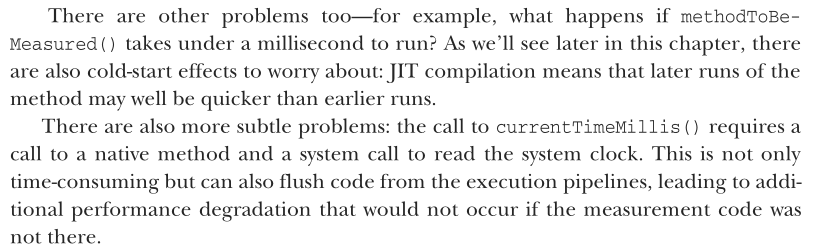
This will produce an output line that should give a millisecond-accurate view of how long methodToBeMeasured() took to run. The inconvenient part is that code like this has to be added throughout the codebase, and as the number of measurements grows, it becomes difficult to avoid being swamped with data.
Automatic instrumentation via Class Loading
This is the mechanism that allows APM (Application Performance Monitoring) tools to profile and trace Java applications without modifying their source code.
Instead of forcing developers to manually add timing code around every method, the JVM allows code to be modified at load time:
Bytecode Interception: When the JVM's class loader reads a compiled
.classfile into memory, an agent (usually registered via-javaagent:agent.jar) intercepts the raw bytecode before the class is finalized.Bytecode Injection: The agent modifies the bytecode directly using libraries like Byte Buddy or ASM. It injects instructions at:
Method entry: records a start timestamp (
System.nanoTime()).Method exit / exception handler: records the exit timestamp and computes the elapsed duration (tend−tstart).
Decoupled Data Export: The measured durations, method names, and execution metadata are written to an in-memory, thread-safe buffer or ring buffer. Background worker threads then consume this buffer asynchronously to write to logs or transmit the metrics over the network (e.g., via gRPC/HTTP), keeping instrumentation overhead on the application threads minimal.

Know what your performance goals are, in most cases, this should be a simple and precisely stated goal, such as the following?
Just as important as knowing what to measure is knowing and communicating the end goal of tuning. In most cases, this should be a simple and precisely stated goal, such as the following:
Reduce the 90th percentile end-to-end latency by 20% at 10 concurrent users
Reduce the mean latency of handleRequest() by 40%

Know when to stop!
Here’s a set of very simple guidelines for knowing what to optimize. You may need to adapt these for your particular circumstances, but they work well for a wide range of situations:
Optimize what matters, not what is easy to optimize.
Hit the most important (usually the most often called) methods first.
Take low-hanging fruit as you come across it, but be aware of how often the code that it represents is called.
At the end, do another round of measurement. If you haven’t hit your performance goals, take stock. Look and see how close you are to hitting those goals, and whether the gains you’ve made have had the desired impact on overall performance.
What are the key concepts and limitations of measuring time in Java performance tuning?
Core Principle: Effective performance tuning requires understanding how to interpret execution timings and recognizing the inherent limitations of the platform's clocks.
Key Takeaways for Java Timing Systems:
Systems contain multiple internal clocks.
Millisecond-level timings are generally safe and reliable.
Higher-precision timings require careful handling to avoid clock drift.

What does the Java process consist of?
The standard Java process has both a stack and a heap.
The stack is where local variables are stored. Local variables that hold primitives directly store the primitive value in the stack.
On the other hand, local variables of reference type will point at a location in Java’s heap, which is where the objects will actually be created.
Figure 7.4 shows where storage for variables of various types is located.

Areas of memory - (before JDK 27)
The JVM has the following different areas of memory that are used to store objects during their natural life cycle:
Eden—Eden is the area of the heap where all objects are initially allocated, and for many objects, this will be the only part of memory in which they ever reside.
Survivor—These spaces are where objects that survive a garbage collection cycle (hence the name) are moved. Initially they are moved from Eden, but they may also move between survivor spaces during subsequent GCs.
The Old generation (also called the Tenured generation) is the area of the JVM heap reserved for long-lived objects—data that has survived multiple Young garbage collection cycles and is expected to remain in memory for an extended period.
What are the main logical areas (regions) of the JVM heap during an object's lifecycle in modern Java (JDK 27 default G1 GC), and how do they interact with collectin - (from JDK 27)
Heap Structure (Region-Based): Under JDK 27's universal default G1 GC, the heap is divided into flexible regions (rather than fixed contiguous blocks) that dynamically change roles:
Eden Regions:
Where almost all new objects are initially allocated.
Exception: Humongous objects (≥50% of a region's size) bypass Eden and are allocated directly into the Old generation.
Survivor Regions:
Hold objects that survive a young collection (evacuated from Eden or earlier Survivor regions) so they can "age" before promotion.
Rather than two fixed
S0/S1partitions, G1 dynamically allocates fresh Survivor regions on demand during each collection.
Old (Tenured) & Humongous Regions:
Store long-lived objects promoted out of Survivor regions once they reach the tenuring threshold, plus newly allocated Humongous objects.
Collection Behavior: While Young-only collections skip standard Old regions, Old-generation memory is reclaimed during Mixed collections (which collect Young regions + candidate Old regions), and unreferenced Humongous regions can be reclaimed during any young pause.
What is the purpose of survivor regions in Java Garbage Collection (JDK 27 default G1 GC),
and what types of collections stem from the generational hypothesis?
Role of Survivor Regions:
Act as a catch-all aging buffer so that short-lived objects created immediately before a garbage collection cycle are evacuated and given time to die rather than immediately promoted.
What Happens Without Survivor Regions (Premature Promotion):
Very recently created (yet short-lived) objects would still be reachable during a collection, causing the GC to mark them as "live" and promote them directly into the Old (Tenured) generation.
Once promoted, those objects quickly die while continuing to waste Old-generation space until the next Old-region cleanup.
This unnecessary buildup forces more frequent Old-generation collections and increases GC overhead.
Collection Types in Modern Java (JDK 27 Default G1 GC):
Young-Only Collection: Collects dead objects within Young regions (Eden and Survivor) and opportunistically reclaims dead Humongous regions.
Mixed Collection: Collects all Young regions plus candidate Old-generation regions with the highest garbage ratio (the standard way Old space is reclaimed).
Full Collection (Fallback): A disruptive whole-heap collection triggered only as a last resort if concurrent collection cannot keep up with memory allocation.
A young collection attempts to clear the “young” spaces (Eden and survivor). The process is relatively simple, as described next:
All live young objects found during the marking phase are moved.
Objects that are sufficiently old (those that have survived enough previous GC runs) go into Tenured.
All other young, live objects go into an empty survivor space.
At the end, Eden and any recently vacated survivor spaces are ready to be overwritten and reused, because they contain nothing but garbage.

When does Full collections happen?
When a young collection can’t promote an object to Tenured (due to lack of space), a full collection is triggered.
Depending on the collector used, this may involve moving around objects within the old generation. This is done to ensure that the old generation has enough space to allocate a large object if necessary. This is called compacting.
What are Safepoints?
A specific point in program execution where a thread's state (registers, stack pointers, and heap references) is completely known and consistent, allowing the JVM to safely inspect or modify memory without concurrent mutation from application code.
Why G1 is Regionalized?
G1 is Regionalized, which means that the G1 Java heap divides the heap into equal-sized regions (such as 1, 2, or 4 MB each). Generations still exist, but they are now no longer necessarily contiguous in memory.
Regionalization has been introduced to support the idea of predictability of GC pauses.
The new arrangement of equal-sized regions in the heap is illustrated in figure 7.6.

How does G1 GC collect the Old generation (covering IHOP, concurrent marking, and mixed collections)?
Why Old Collections Differ: Old-generation objects tend to live much longer, and the Old generation is significantly larger than the Young generation.
Trigger (
IHOP): G1 monitors Old-generation occupancy; once it fills past the InitiatingHeapOccupancyPercent (IHOP) threshold (which defaults to 45% before adaptive tuning), an Old collection cycle begins.Phase 1 — Concurrent Marking: Runs mostly concurrently alongside application threads (based on the Dijkstra-Lamport marking algorithm) to identify live objects and calculate how much garbage exists in each Old region.
Phase 2 — Young + Mixed Collections:
Once concurrent marking finishes, a Young collection runs, followed by Mixed collections.
Mixed collections evacuate Young regions plus the Old regions containing the highest amount of garbage, copying surviving Old objects into fresh Old regions (compacting them in the process).
What happens if G1 cannot reclaim the entire Old generation in a single cycle, and when does it fall back to a Full GC?
Incremental Collection: If the entire Old generation cannot be collected in one cycle, G1 simply collects a subset of candidate regions, ends the cycle, and releases GC CPU cores back to the application—continuing over subsequent cycles.
Steady State: As long as long-lived object allocation does not permanently outpace reclamation, the application runs smoothly without whole-heap pauses.
Last-Resort Full GC Fallback: If allocation outstrips reclamation for a sustained period, G1 triggers a disruptive, Stop-The-World (STW) Full GC to clean and compact the entire Old generation (typically only seen when an application is severely overloaded or misconfigured).
What are "humongous" objects in G1 GC, how are they allocated, and how can they trigger a Full GC?
Definition: Objects that exceed a single region's threshold (specifically >= 50% of a G1 region's size, such as large primitive/byte arrays; in classic 1 MB regions, anything over ~512 KB–1 MB).
Allocation Rules: Because large arrays require contiguous memory, G1 converts a set of adjacent free regions into a single humongous region (part of the Old generation).
Fragmentation & Full GC: If the heap lacks enough adjacent free regions to satisfy a humongous allocation—even after running a Young collection—the heap is fragmented, forcing G1 to run a STW Full compacting GC to consolidate free space.