ECON 252 Exam 1

Cost-benefit

Pursue a choice only if the benefits are greater than or equal to the cost

Opportunity cost

The true cost of anything that is the next-best alternative given up

Marginality

Break “how many?” into a series of “one more?” decisions

Compares marginal benefit to marginal cost → go until they are equal

Interdependencies

Your best choice depends on other choices, markets, and expectations

Intertemporal Budget Constraint

(1+r)y1+y2=(1+r)c1+c2, c=consumption, this equation is measured in period 2 $

r=interest, inc r steepens budget line, dec r flattens budget line

y=income, inc y shifts the budget line outward, dec y shifts the line inward

E is where consumption equals income, always sits on the budget line, which is determined by r

E is always affordable, so the budget line pivots at E (y1,y2)

left of E (c1>y1) → saver, sacrificing period 1 consumption for period 2 consumption

right of E(c1>y1) → borrower, sacrificing period 2 consumption for period 1 consumption

lifetime wealth=m=y1+(y2/1+r)=present value of income

Quantity demanded

the amount of a good a buyer plans to purchase at a given price

Demand

describes quantity demanded at every price

reflects both willingness to pay and ability to pay

Market Demand- total quantity demanded by everyone in the market at each price

Law of demand

as prices falls, quantity demanded rises, aee, and vice versa

price change → movement along demand curve

Demand shifters

Shift the whole demand curve

Income:

-Normal goods: inc income → inc demand (buy more stuff when rcher)

-Inferior goods: inc income → dec demand (buy better stuff when richer)

Related Goods:

-Substitutes: inc price of sub → inc demand for good

-Complements: inc price of comp → dec demand for good

Preferences/tastes- trends change desire for a good

Expected future prices- buy more today if more expensive tomorrow and vice versa

Number of buyers- more buyers → inc demand

Demand Elasticity

Slope of demand is related to elasticity

Elastic goods- goods that have close substitutes ex. chips

Inelastic goods- goods that do not have close substitutes ex. gas

inc price of inelastic good → dec demand of elastic good

Quantity supplied

The amount a seller plans to sell at a given price

Supply

Described quantity supplied at every price

Market supply- total quantity supplied by everyone in the market at each price

Law of Supply

As price inc, quantity supplied rises, aee, and vice versa

Price change → movement along the supply curve

Supply Shifters

Shift the whole supply curve

Input prices inc → marginal cost inc → supply dec

Technology improves → marginal cost dec → supply inc

Expected future prices- expect higher prices tomorrow, sell less today → supply falls

Number of sellers- more sellers → supply inc

Government policy:

-taxes raise effective marginal cost → supply dec

-subsidies lower effective marginal cost → supply inc

Equilibrium

Where supply meets demand(P*=Q*)

Surplus

At P1>P*, quantity supplied exceeds quantity demanded

Sellers respond by cutting prices, market →P*

Consumer surplus- the gap between what a buyer is willing to pay and what they actually pay (below demand curve, above market price)

Producer surplus- the gap between what a seller receives and their marginal cost of producing it (above supply curve, below market price)

Shortage

At P2<P*, quantity demanded exceeds quantity supplied

Buyers bid the prices up, market → P*

Efficiency

An outcome is efficient if it maximizes the total surplus available to everyone in the market

At equilibrium, consumer and producer surplus are maximized

Pareto improvement- a change that makes at least one person better off without hurting anyone else

Pareto efficient- an allocation where no Pareto improvement remains possible

Dead Weight Loss

Lost surplus (nobody gets it) due to lost mutually beneficial trades becoming unavailable at certain prices and quantities

Market failure

A situation where the market outcome in not efficient- total surplus left on the table and no price adjustments fix it

Systemic risk

A bank choosing how much leverage and risk to take on weighs its own expected profit and risk of failure- not the cost of failure on the rest of the system

Creates a negative externality- benefits fall on bystanders

Fixes:

-Capital requirements- force banks to find more of their balance sheet with their own money → internalizes downside

-Stress tests

-Capital surcharges-a tax to equal external cost

Asymmetric information

One side cannot verify what the other knows

Fixes:

-Disclosure and regulation- standardized reporting narrows information gap

-Lender of last resort- when private lending freezes, the central bank can lend

Public goods

Non-excludable, no one wants to pay

Non-rival, usage is independent of usage

Left alone, markets underinvest in public goods

Fixes:

-Government provision

Coordination Failure

Households expect a recession and start spending less → lower income and job loss (recession)

Fixes:

-Monetary Policy- lower interest rates make borrowing-financed spending cheaper, pulling consumption and investment forward

-Fiscal policy- government spending or tax cuts can substitute for the lack of private spending

Price Controls

Price ceiling-max price

Price floor-min price

Without price controls, shortages and surpluses can happen in markets

GDP

The market value of all final goods and services produced within a country during a given period of time

Is a FLOW

The Expenditure Approach

Y=C+I+G+NX

Y=output

C=consumption-household spending on goods and services

I=investment-spending on new capital, not buying a stock

G=government spending-purchases of goods and services, transfer payments are excluded (ex. social security)

NX=net exports- exports minus imports

(looks at the demand side of economics)

Production Function

Y=F(K,L)

K=capital

L=labor

(looks at supply side of economics)

Expanded Expenditure Approach

Y=C(Y-T)+I(R)+G+NX

(Y-T) → take home pay, T=taxes

R → real interest rate

Nominal GDP vs. Real GDP

Nominal GDP-output valued at current prices, grows faster due to cumulative inflation

Real GDP-output valued at constant (base-year) prices

GDP Deflator

=(Nominal GDP/Real GDP) x 100

GDP Per Capita

=GDP/population → provides a rough proxy for average income

GDP itself does not reflect how well people are living, just the size of an economy

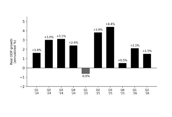
The Business Cycle

Expansion-period of rising GDP

Recession-period of sustained decline

Displayed by the GDP growth chart

The Rule of 70

Divide 70 by the annual growth rate to get the approximate number of years for a quantity to double

Physical Capital

The machines, factories, and infrastructure workers use

More capital per worker raises output per worker

Human Capital

The skills and knowledge embodied in workers themselves, built through education, training, and experience

Production Functions

Y=A*F(K,L) - basic

Y=A*F(K,L,H) - basic w/ human cap

y=A*f(k) - per-worker

A=total factor productivity

K=capital stock

L=labor

F=how capital and labor combine

Returns to Scale

If you scale both K and L by the same factor, λ, what happens to output?

Constant returns: F(λK, λL) = λF(K,L)

Increasing returns- output scales more than proportionally

Decreasing returns-output scales less than proportionally