DTSA 5505
 Call Kai
 Learn
 Practice Test
 Spaced Repetition
 Match
 Flashcards
 Knowt Play
1/51

There's no tags or description
Looks like no tags are added yet.
52 Terms
Information Formula
Info(D) = -Σ pi * log(pi)
Sigma = Sum of
pi = Probability of class Ci = Ci / D
log(pi) = Log of the probability of class Ci
pi Formula
pi = |Ci| / |D|
Ci = # of instances of the i-th answer (Ex. C1 = Approved Applicants, C2 = Denied Applicants)
D = Whole collection of instances (Ex. All the applicants)
Information Formula following Split
InfoA(D) = Σ(|Dj| / |D|) * Info(Dj), where Dj is one pile in the split
It’s the sum of the Information Formula applied to each pile in the split multiplied by their respective weights
Ex. Pile A = 5 (2A, 3D), B = 3 (3,0), C = 4 (2,2)
A = 0.4 * log2(0.4) + 0.6 * log2(0.6) = -0.971, flip the sign and get 0.971
B = 0 because it is pure
C = 1.0 because it is perfectly 50/50
0.971*(5/12) + 0(3/12) + 1(4/12) = 0.738
Gain = Info(D) - InfoA(D) = 0.980 - 0.738 = 0.242
Gain Formula
Info(D) - InfoA(D)
Bayes Theorem
“Chance the guess is right, given what I observed”
(How common the guess is overall) * (How often I’d see this observation if the guess were true) / (How common the observation is overall)
Aka score = likelihood * prior
[P(Ci) * P(X | Ci)] / P(X)
Where Ci is one possible answer (class) like “Picnic = yes/no” and X is the details of that day
We skip dividing by P(X) because both the winner and loser and divided by the same P(X)
Bayes Theorem - Naive Assumption
P( X | Ci) = Π P(xk | Ci)
It is the product of the individual chances of each trait being among picnic days
Example: Overcast, Mild, High Humidity, False (Wind)
Out of 9 picnic days, 4 were O, 4 were M, 3 were H, and 6 were F
P(X | yes) = 4/9 × 4/9 × 3/9 × 6/9 - This is the Likelihood
Take that number, multiply it by the prior to get the score for yes
Laplacian Correction Example
If we have 0 for overcast when looking at Picnic = No, and we add 1 to each count for that trait
Overcast was 0, becomes 1
Rainy was 3, becomes 4
Sunny was 2, becomes 3
So 0/5 becomes 1/8, the denominator updates too
Support Vector Machines
Classification method with supervised learning where the goal is to draw a boundary that separates the classes
In 2D it’s a flat line, in 3D it’s a flat sheet, in more dimensions it’s a hyperplane
Analogy: Two groups of people standing in a field, you put a rope on the ground between them, people on the left are in Group 1, people on the right are in Group 2
Margin
Support Vector Machines (SVMs)
Margin is the distance from the boundary to the nearest points on each side. SVM picks the line with the largest margin, called the maximum margin hyperplane
Why? Because a line squeezed right up against some points is risky. Real data is noisy, so a slightly unusual point could land on the wrong side, so a line with a wide empty buffer on both sides is safer
Support Vectors
Support Vector Machines (SVMs)
Support vectors are the few points sitting right at the edge of the buffer and define the margin
Points far away from the boundary don’t affect where it goes, but if you move one of the support vectors the boundary shifts
This is where the name comes from, it is a machine built from support vectors
Linearly Inseparable
When classes are tangled together along a wavy border, and no single straight line can separate them
This is fixed by adding dimensions
Why does adding dimensions fix data that is linearly inseparable?
You add dimensions by transforming each point into a version with more attributes. In the higher-dimensional space, points get more spread out, and flat boundary may now separate the classes. You then run the normal maximum-margin method in that bigger space
Example: On a number line, we have blue points at -1, 0, and 1, red points at -3 and 3. No single line separates them. If we give each point a second attribute, like it’s value squared, we get (-1,1), (0,0), (1,1), (-3,9), & (3,9), which can be cleanly separated by a line at height 5. The extra dimension did the work
Linearly Inseparable Shortcut: Kernel Trick
Moving every point into a high-dimensional space is expensive. Finding the maximum margin only needs dot products (a way of measuring how similar two points are)
The dot product in the high-dimensional space can be calculated by applying a kernel function to the original points, with no actual transformation needed
Classification vs Clustering: Which is supervised?
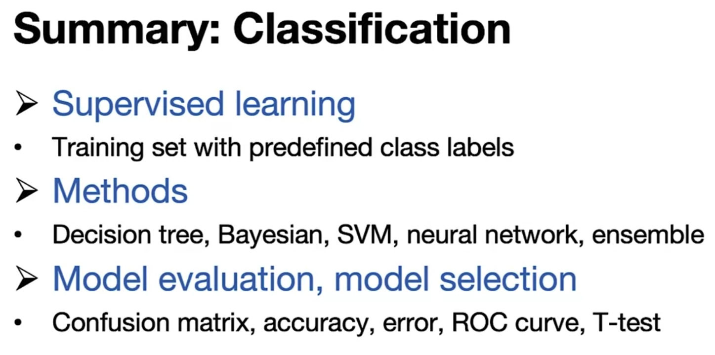
Classification is supervised
Clustering is unsupervised
Decision Tree - Bullet Points
Top-down, Recursive, Attribute Selection, Split
Bayesian Classification - Bullet Points
Probability, Naive Assumption, Belief Network
Classification Methods - Review Slide
Decision Tree Induction: Efficient, Easy to Interpret
Bayesian Classification: Efficient, Explainable, Incremental (If you get new data just update the counts)
Support Vector Machines: Good/High Performance
Neural Networks: Complex, High Performance, Poor Interpretability
Ensemble
Combined use of multiple models
Analogy: Consulting multiple doctors
Bagging: Equal weights, majority voting
- Training set: random sample with replacement
Boosting: Weighted votes (this is when you think certain models are better than others)
- Adjusted weights to focus more on misclassified cases

Model Evaluation
Holdout, random sampling
- Split into training set (for model construction) & test set (80/20)
(k-fold) Cross-validation
- Split into k partitions, each 1 for testing & (k-1) for training
- Divide your data into k segments then do k runs, each time selecting 1 holdout and using the remaining k-1 segments as the training data
Bootstrapping
- .632 Bootstrapping
- Random sample with replacement
Classification Accuracy
Confusion Matrix
- TP, FP, TN, FN
- Maximize TP’s and TN’s, minimize FP’s and FN’s
Classification Accuracy - Measures
Sensitivity: TP / Total Positives
Specificity: TN / Total Negatives
Precision: TP / (TP + FP)
Accuracy: (TP + TN) / (TP + TN + FP + FN)
- On the slide she had Sensitivity(Pos / Pos + Neg) + Specificity(Neg / Pos + Neg)
Costs & Benefits of TP/TN/FP/FN
Depending on the situation you may want to consider which are more important:
If you are dealing with Fraud Detection:
- FP: Normal case flagged as fraud
- FN: Fraud misclassified as normal
Probably want to err on the side of FP’s
When TP/TN/FP/FN doesn’t work
Multi-class Classification
Example: Human Activity Recognition
Model will make errors, but the type of mistake matters: misclassifying one activity as a closely related activity may be far less severe than confusing it with a completely different one
If Activity 1 and 2 are similar, but 1 and 3 are not, misclassifying 1 as 3 is worse than misclassifying 1 as 2. So you would assign different weights or penalties to different types of errors
Big Takeaway: There is not one measure or calculation to compare everybody. You need to understand your scenario and then decide which measure or metrics are more important in that scenario
Big Takeaway on Classification Metrics
There is not one measure or calculation to compare everybody. You need to understand your scenario and then decide which measure or metrics are more important in that scenario
Scoring Number Predictions
When the answer is a number (stock price, temperature, wind speed), an exact hit is nearly impossible, so you score how far off each guess was
She named these measures:
Absolute Error
Squared Error
Mean Absolute Error
Mean Squared Error
Relative Absolute Error
Relative Squared Error
Equations for Scoring Number Predictions

ROC Curve
Across (x-axis): False Positive Rate - FP / All Real Negatives
Up (y-axis): True Positive Rate - TP / All Real Positives
You want to be as far up and as far left as possible
T-Test Formula
t=var(M1−M2)/kerr(M1)−err(M2)
var(M1−M2)=k1i=1∑k[err(M1)i−err(M2)i−(err(M1)−err(M2))]2
T-Test Steps
- Do the k-fold cross-validation
- Calculate t
- Look up the cutoff (need df and significance level, a)
*If doing a two-sided t-test you need to do 1 - a/2
- Compare
If t is bigger than the cutoff, you reject “the models are equal” (t is statistically significant if t > cutoff)
Summary: Classification
What is Clustering?
You have objects described by several attributes, but no predefined categories and no labels. Goal is to discover natural groupings. This is unsupervised learning, in contrast to classification, which is supervised
What are the properties of good clustering?
High intra-cluster similarity (in the same cluster)
Low inter-cluster similarity (between clusters)
What to Judge a Clustering Method On
Quality: Are the clusters good?
Efficiency: Is it fast on large data?
Incremental: When new data arrives, can you update the existing clusters instead of starting over?
Four Questions for Evaluating a Clustering
Clustering Tendency: Does the data have clusters at all? If the points are spread roughly evenly or randomly, no method will find real groups
Cohesion & Separation: Are objects tight inside their cluster (cohesion), and are clusters far apart (separation)? These are the two properties above, made measurable
How many clusters? You usually don’t know the number in advance, and there are measures to compare different numbers
Outside Knowledge: Domain experts may already know roughly how many
clusters to expect, or what good ones look like. Use that
You can also compare two different clusterings of the same data to see which is better
Silhouette Coefficient - What is it, scores, and equation
Measures how well-separated and cohesive your clusters are by comparing how close each data point is to its own cluster versus others. Scores:
Near +1 - P is far closer to its own cluster than to any other (well placed)
Near 0 - P sits on the border between two clusters
Negative - P is closer to another cluster than its own, it’s probably in the wrong one
Equation: (b - a) / the larger of a and b
a = P’s average distance to the other objects in its own cluster
b = P’s average distance to the objects in the other cluster
Example: a = 1, b = 8, (8 - 1) / 8 = 0.875
Five Families of Clustering Methods
Partitioning: Split the N objects directly into a chosen number of clusters
Hierarchical: Build clusters at many levels, by repeatedly merging small ones or splitting big ones
Grid-based: Chop the space into grid cells and see which objects land in which cell
Density-based: Treat crowded regions as clusters
Probabilistic: Each object belongs to each cluster with some probability (like 70% Cluster 1, 30% Cluster 2) instead of a hard assignment
Closed vs Max Pattern: Example
Closed Pattern means there is no super pattern with the same support, Max Pattern means there is no super pattern that is frequent
Original receipts: bread appears 4 times, milk 3 times, and bread+milk 3 times.
Max keeps: bread+milk. Anything inside it is automatically frequent, so bread and milk need no separate mention. The counts are lost.
Closed keeps: bread (4) and bread+milk (3).
Milk is dropped because bread+milk has the same count (3), so nothing is lost.
Bread is kept because its count (4) differs from bread+milk (3). One receipt had bread without milk, and dropping bread would erase that
Max Pattern: A frequent itemset where no bigger itemset containing it is frequent
Closed Pattern: An itemset where no bigger itemset containing it has the exact same support
Apriori Algorithm
Key idea is pruning: if X is not frequent, then no bigger itemset containing X can be frequent
Analogy: If hardly anyone buys caviar, you don’t need to check “caviar + crackers” or “caviar + lemon” because they can’t be popular either
The steps:
1. Scan dataset to get freq. 1-itemsets
2. Generate Candidates for k+1 itemsets from freq. k-itemsets
3. Scan dataset again to remove infreq. candidate (k+1) itemsets
4. Repeat until no frequent itemsets or candidates are left
Apriori Rules
Self-Joining: To build a k+1 size candidate, combine two frequent groups of size k only if their first k-1 items match
- BC and BE both start with B and differ only at the end, so they join into BCE
- BC and CE don’t share a starting letter, so they don’t join
Pruning: After building a candidate, check that every subset of it is frequent
L3: abc, abd, acd, ace, bcd
- abc + abd -> abcd: Both start with ab, All pieces (abc, abd, acd, bcd) are in L3 → Valid candidate
- abd + acd: Don’t start the same, Rule 2: Not checked → Skipped, it would only recreate abcd, a duplicate
- acd + ace -> acde: Both start with ac, Not all pieces (acd, ace, ade, cde) are in L3 → Pruned before counting
Why Apriori is Slow
Multiple scans of the whole dataset
It builds a lot of candidates - Every round creates new possible combinations
It has to check the Support of all candidates by going back through the database
Apriori Speed-Ups
Partitioning - A freq. itemset must be freq. in at least one partition (can parallelize)
Sampling - Random sampled subsets are likely to contain freq. itemsets
Transaction Reduction - Remove Ti if it doesn’t contain any freq. k-itemset
Hash Tree
Vertical Data Format (Flipping the table around)
Support Counting using Hash-Tree
Steps
Create Subset Function - Sets up a Hash Tree where the rules are 1,4,7 go left, 2,5,8 go middle, and 3,6,9 go right
Create Tree Using Subset Function - Run all possible candidates through your tree, this establishes your leaf nodes
Run every transaction, Ti, through the tree
Generate the k-item subsets for the transaction. For a 5-item transaction and k = 3, that gives 10 subsets
Traverse the tree with each subset, hashing its items in order to follow a path down
Check the leaf. If the path ends at a leaf that holds a matching candidate, add 1 to that candidate’s counter
The candidates in the 3-itemset tree are all the freq 2-itemsets that combined and passed the Join and Pruning rules

Vertical Data Format

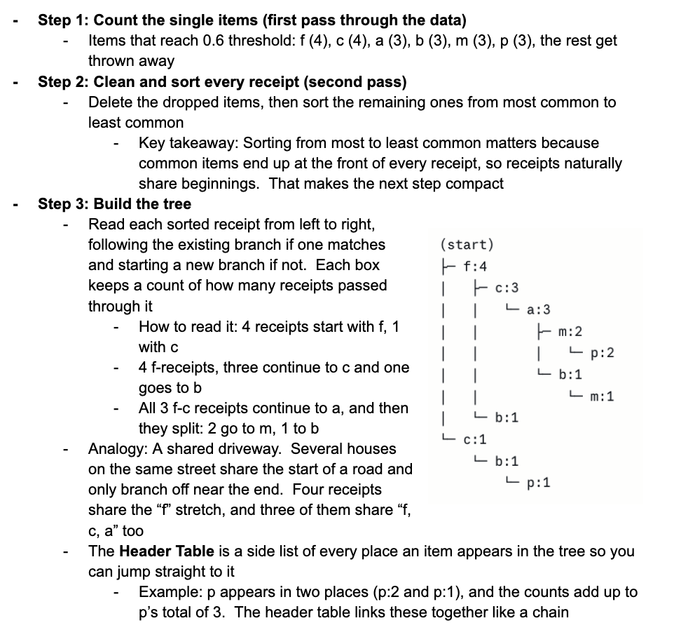
FP-Growth
Asks whether we can skip candidates altogether and only build combinations we already know are frequent
Analogy: Apriori is trying every key on your key ring, FP-growth is like looking at the lock first and only checking keys that could possibly work
FP-Growth Algorithm
If d is freq. in the database conditioned on abc, then abcd is freq
If the cut off is 100 out of 1000 transactions and abc is in 150, and then d is in 110 of those, then not only is d frequent, so is the combination of abcd
Grows patterns using local frequency items
Find frequent itemsets without candidate generation
Using the FP-Growth Tree

Association Rules
Frequent combinations only tell you things appeared together, an association rule goes one step further and says “if X is on the receipt, then Y probably is too”
Analogy: A frequent combination says “bread and butter are often bought together.” A rule says “people who buy bread usually buy butter,” and that’s the sentence a store could act on with a recommendation
Association Rule: The Two Scores
Support: P(X U Y), How often do X and Y show up together?
Calculation: Receipts with both / all receipts
Directional? No, the same both ways
Confidence: P(Y | X), When X is there, how often is Y too?
Calculation: Receipts with both / receipts with X
Directional? Yes, changes with direction
What are the 4 Data Mining Methods?
Frequent Pattern Analysis
Classification
Clustering
Anomaly Detection
Originally motivated by Market Basket Analysis