Models

Review: Distributions

• Any random quantity has a probability distribution:

  • all possible values it can take

  • The probability it takes each value

• After repeated draws, it has an empirical distribution

  • all observed values it took

  • The proportion of times it took each value

• After many independent draws, the empirical distribution look more and more like the probability distribution

Models

• a model is a set of assumptions about the data

• In data science, many models involve randomness

  • “Chance models”

• Key question: does the model fit the data?

Approach to Assessment

• if we can simulate data according to the assumptions of the model, we can learn what the model predicts

• we can then compare the predictions to the data that were observed

• if the data and the model’s predictions are not consistent, that is evidence against the model

Sample at Random from a Categorical Distribution

sample_proportions(sample_size, pop_distribution)

• sample at random from the population

  • returns an array containing the empirical distribution of the categories in the sample

Example: Mendal’s Peas

• pea plant of a particular kind

• Each one has either purple flower or white flowers

• Mendal’s model:

  • each plant is purple-flowering with chance 75%

  • regardless of the color of the other plants

Question:

• is the model good, or not?

Choosing a Statistic

• take a sample, see what percent are purple-flowering

• if the percent is much larger or much smaller than 75, that is evidence against the model

  • Distance from 75 is the key

• Statistic:

  • | sample percent of purple-flowering plant -75 |

  • if the statistic is large, that is evidence against the model

Model and Alternative (ex: jury selection & Genetics)

Jury selection:

• Model: The people of the jury panels were selected at random from the eligible population

• Alternative: no, they were biased against black men

Genetics:

• Model: Each plant has a 75% chance of having purple flowers

• Alternative: No, it doesn’t

Steps in Assessing a Model

• Choose a statistic to measure discrepancy between model and data

• Simulates the statistic under the model’s assumptions

• Compare the data to the model’s predictions:

  • Draw a histogram of simulates values of the statistic

  • compute the observed statistic from the real sample

• If the observed statistic: is far from the histogram, that is evidence against the model

A Model of Random Selection: Jury

Model: is that the panel was selected at random and ended up with a small number of black panelist due to chance

Assessing model:

• we can simulate data based on the model. That is, we can simulate drawing at random from a population of whom 26% are Black

• our simulation will show what a panel would be if it were selected at random

• We can then compare the results of the simulation with the composition of an actual jury panel

• if the results of our simulation are not consistent with the composition of the panel in the trial

Continued: The Statistic

First, we have to choose a statistic to simulate. The Statistic has to be able to help us decide between the model and alternative views about the data. The model says the panel was drawn at random from the eligible population. The alternative viewpoint is the case for Robert Swain, which is that the panel contained too few Black panelist to have been down at random.

A natural statistic, is the number or count of Black panelist in the sample. NOTE: small values of the statistic all favor Robert Swain viewpoint.

Continued: Simulating the Statistic Under the Model

If the model were true, how big would the Statistic Typically be? To answer that, we will the statistic under the assumption of random selection and look at the distribution of the results

Continued: Simulating one Value of the Statistic

We can use sample_proportion to simulate one value of the statistic. The sample size is 100, the size of the panel. The distribution from which we will sample is the distribution in the population of eligible jurors.

Since 26% of them were Black, we will sample from the distribution specified by the proportion [0.26, 0.74]

sample_size = 100

eligible_population = [0.26,0.74]

Note: The categories in the output array of sample_proportions are in the same order as in the input array. So the proportion of Black panelist in the random sample is item(0) of the output array.

sample_proportons(sample_size, eligible_popoulation). item(0)

The count in each category is the sample size times the corresponding proportion. So we can just as easily simulate counts instead of proportions.

Let’s define the function that does this.

The function will draw a panel at random and return the number of panelist that were Black

def one_simulated_count():

return sample_size * sample_proportions(sample_size, eligible_population).item(0)

Continued: Simulating Multiple Values of the Statistic

The focus of our analysis is the varibility in the counts. Lets generate 10,000 simulated values of the count and see how they very. As usual , we do this by using a for loop and collecting all the simulated counts in an array.

count = make_array()

repetitions = 10000

for i in np.arange(repetitions):

counts = np.append(count, one_simulated_count)

Continued: Interpreting Results of or simulation (Empirical histogram )

Table().with_column('Count in a Random Sample', counts
).hist(bins = np.arange(5.5, 46.6, 1))

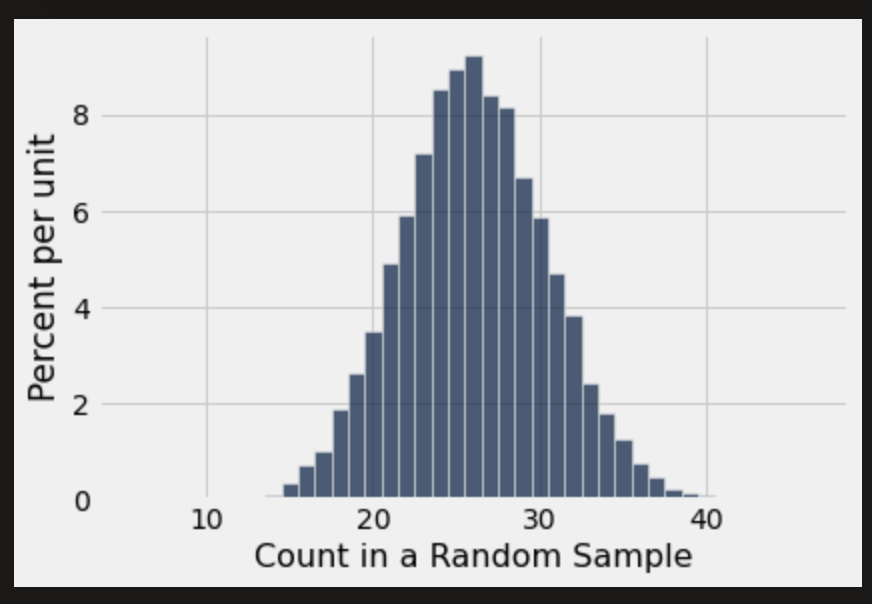
The histogram shows us what the model of random selection predicts about our statistic, the number of Black panelist in the sample

To generate each simulated count, we drew 100 times at random from a population in which 26% were black. So, as you would expect, most of the simulates counts are around 26. They are not exactly 26: there is some variation. The counts range from 15 to about 40.

Continued: Comparing the Prection and the Data

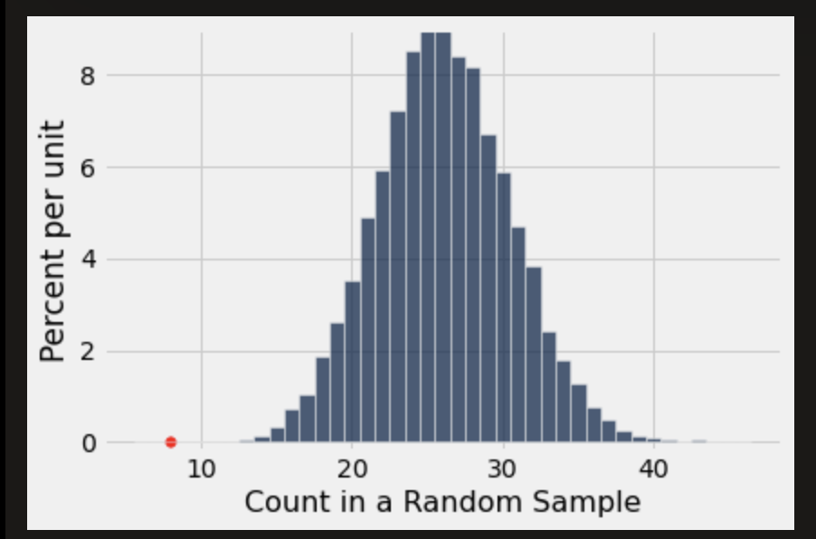
In the panel selected for the trial, there were eight Black panelist. The histogram of simulated counts is redrawn below with eight shows as a RED dot on the horizontal axis. The dot is very far out in the left hand tail of the histogram. Very few of the 10,000 counts simulated by random selection came out to be eight or less

The graph is a visual display of bias in the selection process. It shows that if we selected a panel of size 100 at random from the eligible population, we are very unlikely to get counts of Black panelist that are as low as the eight that were observed on the panel in the trail.

This is evidence that the model of random selection of the jurors in the panel is not consistent with the data from the panel, While it is Possible that the panel could have been generated by chance, our simulation demonstrates that it is hugely unlikely

When the data and a model are inconsistent, the model is hard to justify. After all, the data are real. The model is just a set of assumptions. When assumptions are at odds with reality, we must question those assumptions.

The most reasonable conclusion is that the jury panels was not selected by random sampling from the population of eligible jurors.