STAT210

most of these flashcards are ridiculously long, it's moreso to get all the info about stuff grouped together and easier to find than how lectures are structured

(prac) Common goals of stats

Learn about pop from sample (sample design and representativeness), understand causal effects (experiments and treatment comparisons), learning from observations, ethical and responsible analysis underpins

(prac kinda?) What to consider when collecting data

Specific pop of interest, logistics (how to efficiently sample, sampling units vs measurement units), does sample reflect population, are groups comparable to each other other than independent variable

(prac) Sampling units vs measurement units

Sampling units: unit selected by the sampling design (e.g. quadrats in cockle study)

Measurement units: unit on which measurements are recorded (e.g. cockles)

(prac) 3 main types of studies + overview of each

Surveys: Sample pop to describe pop characteristics, researcher controls how sample collected

Experiments: Establish causal relationships by assigning treatments to experimental units, experimenter controls selection of experimental units, which treatments to assign, randomisation and replication

Observational studies: Investigate relationships between variables as occur in nature, researcher only controls what data included and how data analysed

Outline common themes of all study types

Scope of inference: How will study translate to real world, how far can it scale

Reducing effects of variation: clever design for more precision at same cost/sample size, collect data well, check if data of any other covariates can be collected

Avoiding bias: How to have representative sample in survey or conduct relevant experiment, how can use observational data most appropriately

Why does sampling design matter?

Determines whether and how measurements from sample can be generalised to pop (and how strongly)

Poor sampling cannot be fixed by analysis

(prac) What is probabilistic sampling (probabilistic sampling schemes)

Every unit has known, nonzero chance of selection (justifies extrapolation from sample to pop). Sampling design info should be treated like data.

What does non-probabilistic sample methods rely on?

Untestable assumptions when extrapolating to pop (assumes sample is representative even tho likely not)

List 3 common ways sampling studies fail

Mismatch between sample and pop of interest

Unknown and unequal selection probabilities

Nonresponse/missingness

Population of interest vs sampling frame

Population of interest: Group we want to draw conclusions about

Sampling frame: The list or mechanism from which sample is drawn

If sampling frame does not cover pop of interest, some units may have 0 probability of selection.

List 3 types of bias in sampling

Selection bias, nonresponse bias (missingness), response bias

Outline selection bias

Occurs when some units in pop have zero or systematically different chances of being included in sample, and this is related to the outcome of interest (makes sample not representative).

Outline selection bias risk

Occurs when selection probabilities are unknown or unequal, so bias cannot be ruled out (e.g. in voluntary response samples), so inference relies on untestable assumptions.

Outline nonresponse bias (aka missingness)

Occurs when units that were selected for the sample are not observed, so realised sample differs from intended design (e.g. people drop out of study, animals/plants not detected)

Matters when probability of being observed is related to outcome of interest.

Results in sample not representative of population, and biassed estimated (even with large sample size)

Outline response bias

Aka information or measurement bias. When response/measurement from a unit is systematically biassed/incorrect.

Issue due to measurement (which values recorded), not sampling (which data collected)

e.g. lying on surveys, faulty instruments.

List 3 common sampling designs

Simple random sampling, stratified sampling, cluster (or multistage) sampling

Outline simple random sampling

Every unit in population has equal chance of selection. Conceptual benchmark for inference. Rarely achievable in practice.

Outline stratified sampling

Population divided into known subgroups/strata, samples taken within each stratum (can have each represented proportional to size). Improves precision and ensures representation.

Outline cluster (or multistage) sampling)

Population divded into natural groups (clusters), some clusters sampled (random simple, single-stage), then units within them can also be sampled(2-stage). Logistically efficient but introduces dependence (measurements within clusters typically more similar than to other clusters).

Usually cheaper and less precise than simple random sample or stratified sample of same size (can compensate by taking larger sample)

Multiple levels of variation: cluster-to-cluster and within-cluster variation.

Outline randomisation in experiments

After controlling for other sources of variation, randomly assign experimental units to treatments. Crucial to establishing causal relationships by making groups comparable on average.

(prac) Factors vs levels vs treatments vs experimental units in experiments

Factors = individual variables being manipulated

Levels = values of factors used in experiement

Treatments = different combos of levels for factors (usually includes control treatment)

prac: Experimental units = the physical units given a particular treatments (independent replicates, treatments assigned independently, units same except for treatment)

Outline replication

When 2 or more experimental units are assigned to a given treatment. Helps establish reproducibility, robustness against diverging results, experimental error/uncertainty, amount of precision (experimental error decreases as number of replicates increases).

Key component of establishing valid experimental results and improving precision.

Experimental units vs measurement units

Experimental unit: where manipulation occurs (e.g. different teaching practices)

Measurement units: where measurement occurs, aka observation unit (e.g. tests given to children)

For multi-factor experiments, common to have different levels of experimental units.

What can lead to pseudoreplication

If measurement units are treated as experimental units — not all observations independent, should be treated as such.

List key features of experiments

Randomisation, replication, control or reference group (sometimes)

List key features of observational data

No control over which factors assigned to which sampling units, higher risk of confounding/weaker inference, correlation is not causation, can improve inferences through prior predictions of effects and careful study design

Outline confounding

Occurs when a 3rd variable influences both the treatment/exposure and the outcome (both x and y), creating a misleading association. Large sample sizes do not remove confounding, only make biased estimates more precise.

Where do data come from?

Data produced, not discovered. Result from design decisions, measurement tools, human effort, logistical constraints.

List 2 other data generating processes (other than experiments/observational/surveys)

Administrative/operational data, digital/platform/sensory data

Outline administrative/operational data (examples, key features, risks)

Electronic health records, insurance claims, gov registries — data collected for another purpose.

Key features: collected for operations, not research. Hard-coded categories we can’t control. Changing definitions over time. Often very large.

Stat risks: Misclassification, structural bias, missingness not random.

Outline digital/platform/sensory data (examples, key features, challenges)

Wearables, mobile phone GPS, website log data, satellite measurements

Key features: Automated, high frequency, potentially massive volume, algorithm-mediated measurement

New challenges: Device accuracy varies, firmware/software updates can change measurement, unknown preprocessing.

Sandbox vs standalone dataset

Sandbox = workspace, messy, designed for exploration

Dataset = product, clean, designed for reuse

Importance of data dictionary

Defines variables, specifies units, has description of measurement. Is metadata (data about the data) — without this, analysis is guesswork. Makes data reproducible and transparent.

How to estimate mean of normally distributed data

data from a Normal distribution with mean µ and variance σ^2, X ∼ N(µ, σ^2 )

to estimate mean (mu-hat):

Multiplier for finding confidence interval of estimated mean of normally distributed daya

T-multiplier

Parameter vs statistics

Parameter: An unknown feature of the data-generating process (e.g. µ (true mean) for a population). Can only be estimated

Statistics: A function of the observed data — sample value (e.g. x-bar (sample mean) for data collected). Can be calculated from data. A random variable if data is random variables.

What is a point estimate

Our best estimate for a parameter.

Derived from statistics, e.g. an estimate for the parameter µ (population mean) is the statistic x-bar (sample mean); σ (population standard deviation) is estimated by s (sample standard deviation) — samples used to estimate parameters

Accuracy and prevision are important properties

Accuracy vs precision

Accuracy: On average, does the estimate hit the target (match the true value)

Precision: How much does the estimate vary from sample to sample

What is the sampling distribution

The distribution of a statistic (e.g. sample mean) across repeated samples drawn from the same data-generating process.

What is standard error

The standard deviation of a statistic’s sampling distribution, e.g., σ/√ n is the standard error for the mean

Can almost always estimate the standard error, e.g. the estimated standard error for the mean is s/ √ n (s is sample standard deviation).

What are confidence intervals

A range of parameter values that are consistent with the observed data (given a specified statistical model and study design).

Constructed using the sampling distribution implied by the model and design.

A 95% confidence interval is designed so that, under repeated studies conducted in the same way, 95% of such intervals would contain the true parameter value.

Not all CIs behave as claimed (coverage)

What is coverage of confidence intervals

The long-run proportion of intervals that contain the true parameter value, may differ from the nominal/claimed level.

If coverage greater than nominal rate (e.g. 95% CI), the interval is conservative (over-cover). If coverage lower, interval is anti-conservative (under-cover).

Estimating the population mean of normally distributed data

Confidence interval estimate ± multiplier × standard error

The 1 − α confidence interval formula for µ is x-bar ± t(1−α/2,n−1)s/ √ n

R code: If data in vector called x, use t.test(x)

Use t-multiplier to account for uncertainty due to estimating σ by s (sample standard deviation). For large n, t-multiplier converges to z. Degrees of freedom n-1 to estimate σ since we estimated µ.

Degrees of freedom in t-multiplier for estimating population mean of normally distributed data

Degrees of freedom count how many independent pieces of information are left after estimating parameters other than σ.

Here, we estimated µ (so 1 parameter costs 1 df), leaving n − 1 to estimate σ.

Outline the central limit theorem

Useful for non-normal data.

As n of a sample of independent random variables (which are identically distributed with a mean and finite variance) gets bigger, the data gets closer to normal distribution.

(X-bar − µ) / (σ/√ n) ⇒ N (0, 1)

How to estimate population mean of non-normal data

If n large enough, can use same formula as for normal data — relies on central limit theorom — X values are non-Normal, the sampling distribution for the mean is approximately Normal.

Way to improve skewed data (make more normal)

Can do log-transformations. Downside is operating on the log scale is harder.

Outline binomial proportions (simple model)

X ∼ Binomial(n, p). Estimate p (probability of success) given x (number of successes) and n (number of trials), p-hat = x/n.

Estimate form is estimate ± multiplier × standard error (confidence interval)

R code: use prop.test(x=whatever,n=whatever).

No longer use a t-multiplier (not estimating standard deviation (sigma) anymore as standard error determined by p and n rather than separately estimated).

(prac) Simple linear regression (model_

Images above mean same things in different writing. Models the mean response as a line.

y: response/dependent variable

x: predictor/ independent variable

Beta0: intercept (unknown parameter) — average value of y at x = 0

Beta1: slope (unknown parameter) — average increase in value of y for one unit change in x

ϵ: random errors with normal distribution, mean 0, variance sigma squared (unknown random variable)

Equation above describes variability around the line of best fit (error, assume it’s 0 when we fit the model, so it disappears). Assume are normally distributed with mean 0 and constant variance.

Multiple linear regression

Used when we have multiple predictors (x1, x2, … xk, k = number of predictor variables).

how the average value of an outcome variable depends on linear functions of predictor variables

y: response variable

x1, . . . , xp: p different predictor variables (notation: k also common here)

β0: intercept (unknown parameter)

β1, . . . , βp: slope terms for each predictor (unknown parameters)

ϵ: random error with mean 0 (unknown random variable)

Estimated/expected mean response (fitted model) is:

3 ways to fit a regression model (estimate the parameters so that it fits the observed data well)

Minimise loss: Choose parameters that minimise a loss function (usually based on prediction error, may include penalty terms)

Maximum likelihood: Choose parameters that maximise how probable the data are under a statistical model.

Bayesian inference: Update prior beliefs about parameters using the observed data and a statistical model (parameters not fixed values).

Outline loss functions (ways to fit a regression model)

For each observation there is a residual (difference between actual value versus value estimated by model/line of best fit, measures how far model prediction is from the observed value).

L(ei) used for simple linear regression, assigns a numerical cost to innacurate predictions.

Choose parameters that minimise the total loss.

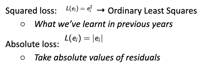
Outline least squares (loss functions, ways to fit a regression model)

Minimise the sum of squared residuals (minimise combined area). Find betahat0 and betahat1 that make sum of squared residuals as small as possible.

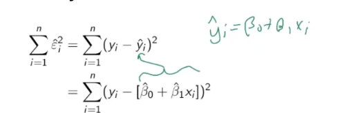
ok idk what any of these equations mean kinda just ignore them ig

Outline maximum likelihood (ways to fit a regression model)

Chooses parameters that make the observed data as likely as possible — maximum likelihood estimation. Maximising likelihood is equivalent to minimising a particular loss function, leads to same fitted line as least squares for many models (including linear regression with normal errors).

Outline Bayesian regression (ways to fit a model)

Combines probability model with prior information, produces distribution for the parameters.

Use same probability model for observed data and also specify prior distributions for the parameters. Priors should be plausible based on prior knowledge about the parameters before observing the data or be kept vague.

Outline Bayesian inference (ways to fit a model)

Combines the prior and the likelihood, Posterior ∝ Likelihood × Prior.

Instead of producing a single estimate for a parameter, produces a posterior distribution for each parameter (P(β0, β1, σ | y))

Parameters treated as random variables, uncertainty quantified using posterior distribution.

Simple liner regression stacked equations

Equation applies to every observation

Can stack equations into vectors and matrices

More compactly written as

With X being the design matrix

Design matrix

In the model:

y is vector of observed outcomes

X is the design matrix

β is vector of regression coefficients

ε is vector of random errors.

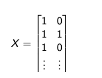
Each column of X corresponds to a predictor variable, each row corresponds to an observation. Regression model determines which columns appear in X.

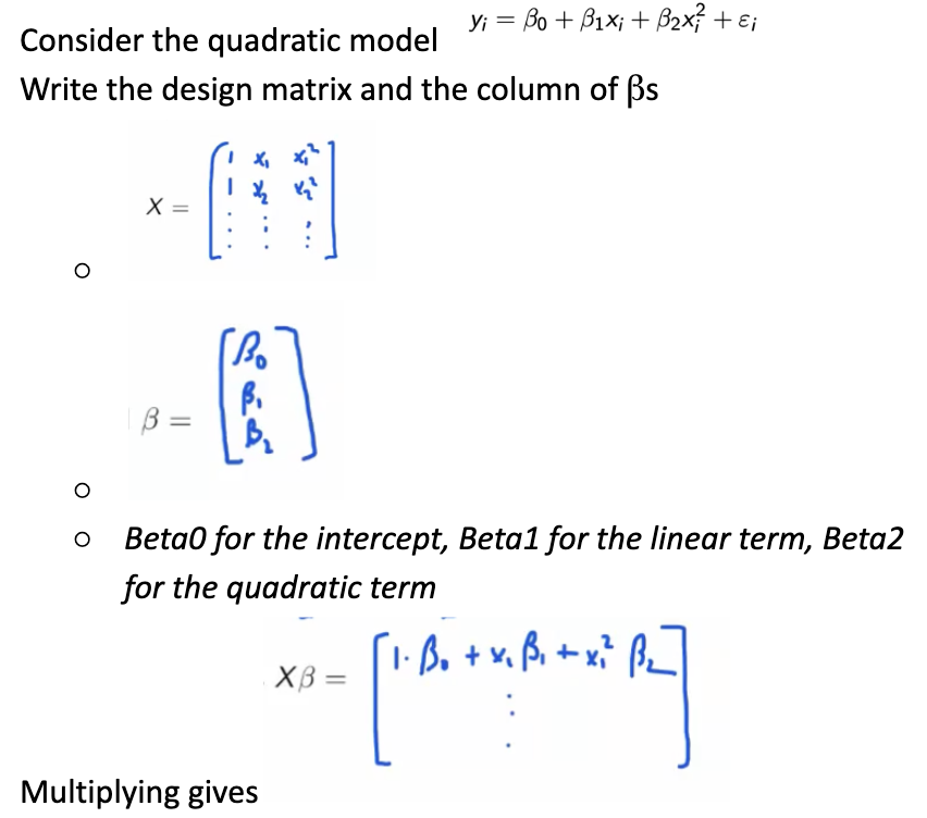
Different Xs (design matrix) for simple linear regression, quadratic regression, and categorical predictor (2 levels)

Simple linear regression:

Quadratic regression:

Categorical predictor (each row = different groups, e.g. 1 0 means not male, 1 1 means male)):

Advantage of writing regression models as y=Xβ + ε

Works for many different regression models

Give general formula for least squares estimates

Helps us understand issues such as multicollinarity.

What is a matrix

Rectangular table of numbers. Dimension of a matrix is the number of rows by the number of columns — e.g. for A: 2 × 3

Matrix addition

Matrices of same size can be added element-wise

Matrix multiplication (matrix x vector)

Each row produces one value — multiply each element of a row by the corresponding element of the vector, and add them all up. Each row = a weighted sum of the vector elements.

Matrix multiplication (matrix x matrix)

Number of columns of first matrix must equal number of rows of 2nd matrix

AB is not the same as BA (except in rare cases)

Transpose of a matrix

Swaps rows and columns

Identity matrix

Behaves like the number 1 for matrices. Is a square matrix (number of rows = number of columns). Can be 2×2, 3×3, etc. Multiplying by the identity does not change a matrix (AI = IA = A)

Matrix inverse

Behaves like division. Multiplying a matrix by its inverse undoes the matrix, turns it into an identity matrix. Only square matrices have inverses. If columns contain redundant info (a column can be constructed from the others as a linear combination), matrix has no inverse.

E.g. if matrix A has inverse A^-1, then:

Matrix for simple linear regression

Mean response is straight line, 1 predictor variable (x), 2 parameters (intercept and slope)

predictor columns in design matrix:

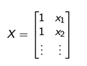
The 1s get multiplied by beta0, so beta0 remains beta0 yk??

Matrix multiplication for quadratic regression

2 components of the linear regression model

1: mean is modelled with a straight line (beta1 is the increase in the average value of y for a one unit change in x, etc, more detail in simple linear regression card)

2: Random variation — error normally distributed, mean 0, constant variance sigma squared, each error assumed to be independent. Small standard variation (sigma) = points close to line, large standard variation = points spread further from line (determines how variable the points are)

Fitted simple linear regression

yhat: fitted value, best guess of value of y for a given x

x: predictor variable

Betahat0: estimated intercept

Betahat1: Estimated slope/effect of x on y

Estimated confidence interval for simple linear regression — R code

confint(modelname) --> intercept and slope

confint(modelname, 2) --> just the slope

if whole interval for beta1 positive, provides evidence of positive association between x and y — e.g. Cheeses with higher levels of H2S tend to have higher taste scores/On average, cheeses with ln H2S values one unit higher tend to have taste scores about 5.78 units higher, We are 95% confident that the true slope lies between 3.84 and 7.71

(prac) R code for estimated values in simple linear regression

lm to make model

summary(model name) (interpreting this is in prac)

e.g.

t-stats and p-values are for hypothesis test (meaning of p-value in prac)

How to make predictions from fitted linear regression

R code

predict(modelname) to make predictions at observed xs

or input model name and list of new xs, e.g.:

Confidence interval for mean response of simple linear regression (2 types of uncertainty)

Estimated value for y given x

untertainty in the regression line (σE(y|x — standard deviation of estimated value of y given x) is due to uncertainty in beta0 and beta1

σE(y|x) increases for x far from estimated x

σE(y|x) becomes small with a large sample size

R code:

Prediction interval for new response Y at x for simple linear regression (2 types of uncertainty)

Uncertainty in the regression parameters and natural variability in data

σY|x (standard deviation of Y given x) goes to σ (standard deviation overall) for large enough n

R code:

Simple linear regression: how to calculate intervals for all xs and add to plots: confidence bands or prediction bands

R code!!

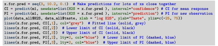
Wide = a lot of natural and/or unexplained variability

Prediction bands can include negative values even if doesnt make sense because model doesnt know the values cant go below zero (e.g. in cheese example)

R² (R squared) in linear regression

Proportion of variance explained. R^2 = 0.5 means that our regression has explained 50% of the variability in the outcome variable.

Useful heuristic but shouldn’t be focused on. Not an objective measure of fit — R² = 0.1 can be good, R² = 0.9 can be bad (but usually bigger value is better), depends on context

Adding important new info can improve R² — in multiple linear regression, more predictors always increases R² even if unrelated, so need substantial increase.

Predictors that span a wider range can explain more variation in multiple linear regression (R² depends on predictors)

A useful heuristic, but take care not to focus too much on R^2: If we add enough variables we will eventually get R^2 = 1.0. The same data-generating process can yield different R^2 depending on the xs

multiple linear regression in matrix form

(prac) Interpreting betas for multiple linear regression

β0 is the average value of y when x1 = x2 = . . . = xp = 0. ( all predictors are zero)

prac: Each βj is the change in the average value of y for a one unit increase in xj all else held fixed (more realistic for experiments than observational data)

Predictions for multiple linear regression

R code: use predict(modelname)

Uncertainty increases when predicting far from the centre of the data (as in SLR)

Uncertainty will decrease if we add useful predictors (MLR cool new feature)

(prac) How to fit models in R (R code)

Use modelname = lm(y ~ x + x2 + etc, data = dataname)

x2 etc only for multiple linear regression, e.g.:

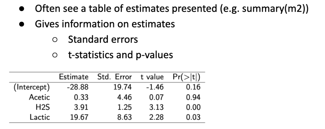
(prac) how to get all beta values (intercept and slopes) for multiple linear regression in R (R code) + confidence interval + summary tables

e.g. “On average, cheeses with Lactic acid values 1% higher have taste scores 19.7 units higher, all else equal.”

conf intervals:

summary table:

Overall F-test for multiple linear regression

Evaluates whether the predictors are related to y — doesn’t establish whether the relationship is important tho

Under H0, the model with predictors does no better than predicting the mean of y than an intercept-only model — The predictors do not explain any more variation in y than expected by chance alone. Fitted model is therefore yhat = yline (best estimate of y is the average of y) in this case.

R code: can find in summary (modelname), gives p-value (Small p-value → strong evidence that at least one predictor is related to y)

F-test does not tell us which predictor(s) are related (look at individual t-tests)

(prac) Assumptions of linear regression

1: Linearity (Average value of y is well described by β0 + β1x — data isn’t curved etc)

2: The errors ϵ are independent (one residual doesn’t tellu s anything about another residual)

3: The errors have constant variance

4: The errors follow a normal distribution

Plot studentised residuals to check (puts on common scale, easier to interpret, should follow an approx normal distribution (specifically a t distribution) if model valid, approx. 68% between -1 and 1, approx. 95% between -2 and 2) — interpreting studentised residual plots is in prac

Residuals in simple linear regression

The true value of y minus the estimated y value. Estimate of the error term ϵi.

Under assumptions residuals should be centered around 0, have no pattern, have constant variance, and be normally distributed (plotted against fitted value y-hat or predictor variable x)

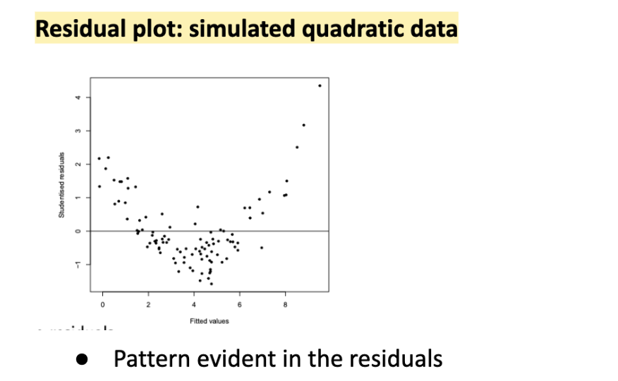
(prac) Checking assumptions of linear regression — 1: Linearity

Critical assumption, describes how 2 variables related, misspecification can lead to incorrect inference.

Violations lead to further violations in assumption 2 (Poor modelling tends to create similar patterns for neighbouring observations).

Pattern in the residuals means a serious departure.

(prac) Checking assumptions of linear regression — 2: The errors are independent

Describes how observations related to one another. Can lead to us finding spurious patterns/relationships. Hard/impossible to diagnose without knowledge of study design.

Pattern in residuals = serious departure

(prac) Checking assumptions of linear regression — 3: The errors have constant variance

Non-constant variance only really a problem if there are major changes in variance. More important when making predictions about future observations (needs to be incorporated)

Serious departure shown by changing residual variance

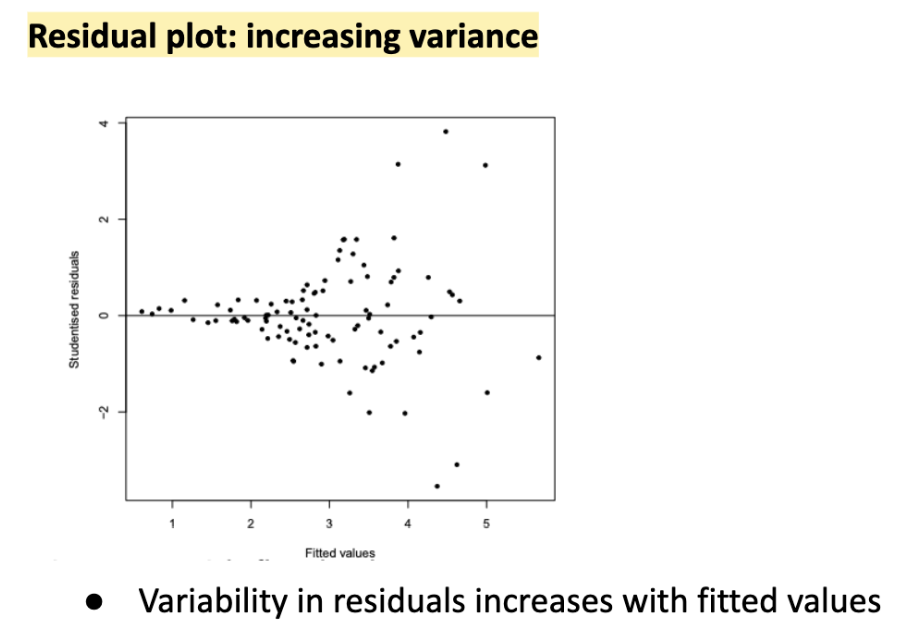
Also often plot the absolute residuals or the square root of the absolute residuals (Easier to see violations of constant variance)

(prac) Checking assumptions of linear regression — 4: The errors follow a normal distribution

Non-normality only a problem if small sample size (exception is outliers/influential points) — central limit theorem kicks in at large sample size. Important for making predictions about future observations (should incorporate when describing how far a new observation might deviate from the line).

Serious departure manifests as non-normal residuals. Can check with Normal quantile-quantile (qq) plots — Residuals are sorted from smallest to largest and compared to the expected sorted distribution from a Normal distribution. Only interested in major departures from normality (outliers — residuals with extreme studentised residuals)

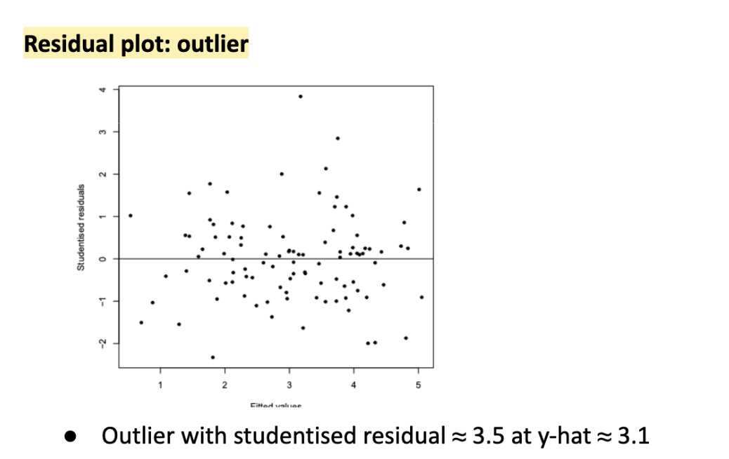
R code for creating residual plots (checking assumptions of linear regression)

Can also get diagnositic plots by plotting an lm model, using plot(modelname)

Influential observations in linear regression

An observation is influential if removing it substantially changes the fitted model. One measure of influence in Cook’s Distance.

2 factors of influence:

• High leverage (unusual predictor values)

  • Occurs when a point has predictor values far from the centre of the data

    • how far x from x-bar in simple linear regression

  • Such points have more potential to affect the fitted regression line

• Large residual (poorly fitted observation)

  •  In simple regression, these are obvious points: outliers with extreme x values

  • In multiple regression, they are harder to identify visually

Observations with both characteristics can strongly affect the model. Inspect observations close to or outside Cook’s Influence contours (dashed lines).

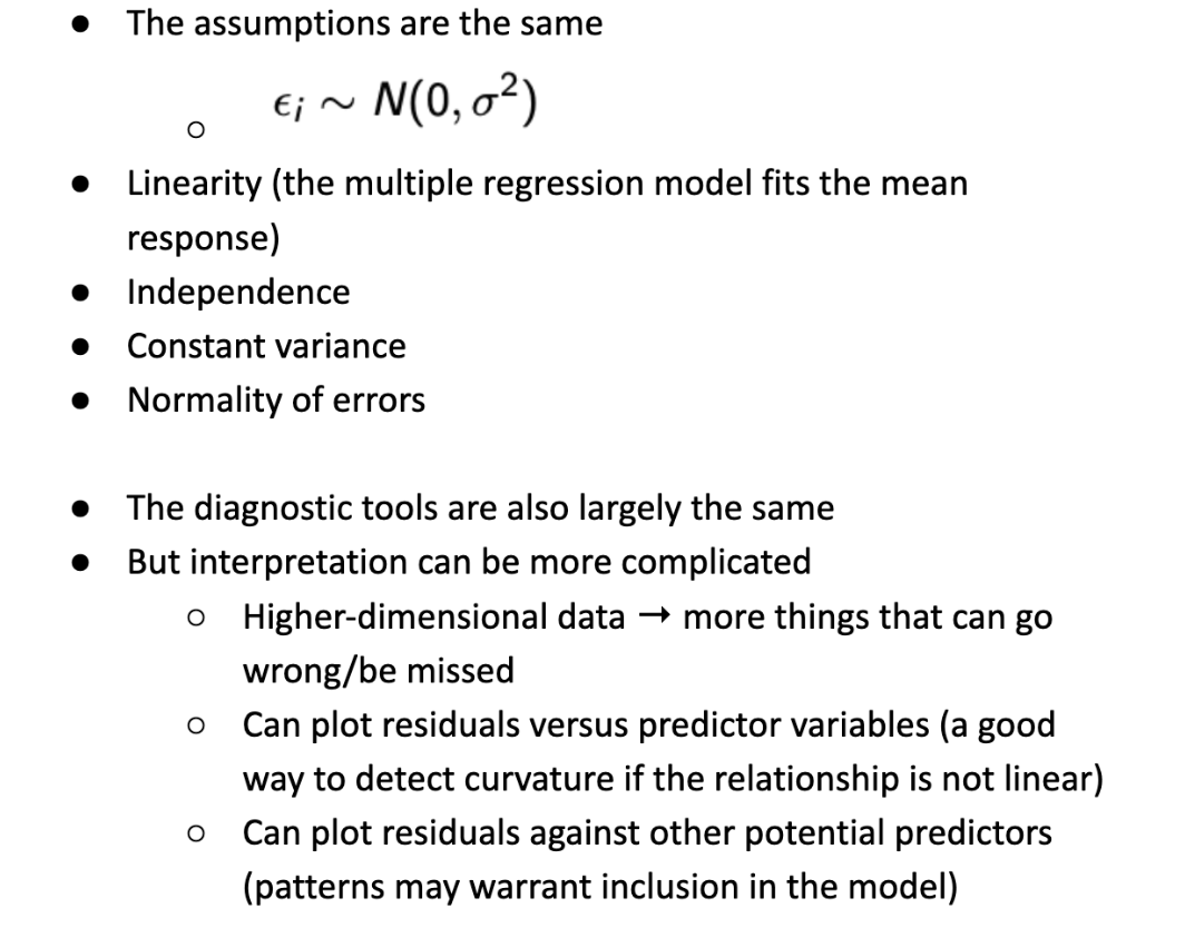
Assumptions/diagnostics in multiple linear regression.

Residual standard deviation

Aka the within-sample root mean squared error (RMSE). Measures typical prediction error (residuals are unexplained variation between estimated and true value). Incorporates inherent variability and things model missed.

To estimate σ^2 we average the squared residuals to get the mean squared error. Assesses model performance of same data used to fit the model — performance for new datasets usually worse (for RMSE and R²).

Unexplained variability in regression model

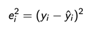
Why are squared residuals bad for estimating the error variance

They’re too small on average because the same data were used to fit the model

What is internal predictive validation

techniques that assess a model’s performance and stability on the same dataset used for development. Identifies overfitting and measures reproducibility

What is external predictive validation

techniques that assess a model’s performance on new, independent datasets. Assesses generalisability to different populations/settings

How to assess internal predictive validation

Leave-one-out-cross-validation (LOOCV). Fit the model without an observation (i), prediction for ith observation based on all observations except itself (yhat(i)). Get prediction error/residual for i value, each e^2(i) (squared residual) estimates squared prediction error for a new observation.

Prediction error combines bias (lack of accuracy) and variance (lack of precision)

(prac) RMSELOOCV

Overall error rate across all observations (root mean square error from LOOCV) — for internal predictive validation